|
1.
|
Select DOE > Mixture Design.
|
|
2.
|
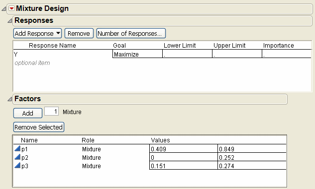
In the Factors panel, use the three default factors but name them p1, p2, and p3, and enter the high and low constraints as shown in Factors and Factor Constraints for the Plasticizer Experiment. Or, load the factors with the Load Factors command in the red triangle on the Mixture Design title bar. To import the factors, open Plastifactors.jmp, found in the Design Experiment sample data folder that was installed with JMP.
|
|
3.
|
Click Continue.
|
|
4.
|
Enter 3 in the Degree text box.
|
|
5.
|
Click Extreme Vertices.
|
|
6.
|
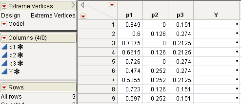
Click Make Table. JMP uses the 9 factor settings to generate a JMP table (Extreme Vertices Mixture Design).
|
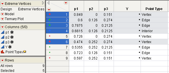
Note: To identify the vertex points and the center (or interior) point, use the sample data script called LabelMixturePoints.jsl in the Sample Scripts folder installed with JMP.
|
8.
|
Run the LabelMixturePoints.jsl to see the results in Identify Vertices and Center Point with Sample Script, and highlight the vertex points and the interior point as shown.
|
|
9.
|
Select Edit > Copy, to copy the selected rows to the clipboard.
|
|
10.
|
|
12.
|
Highlight the new rows and select Edit > Paste to add the duplicate rows to the table.
|
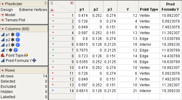
The Plasticizer data with the results (Y values) that Cornell obtained are available in the sample data. Open Plasticizer.jmp in the sample data folder installed with JMP to see this table (Plasticizer.jmp Data Table from the Sample Data Library).
Use the Plasticizer.jmp data from the sample data library (Plasticizer.jmp Data Table from the Sample Data Library) to run the mixture model:
|
1.
|
Select Run Script from the Model red triangle menu in the upper left corner of the data table.
|
|
2.
|
Click Run to see the response surface analysis.
|
|
3.
|
Plasticizer.jmp contains a column called Pred Formula Y. This column was added after the analysis by selecting Save Columns > Prediction Formula from the Response Y red triangle menu.
|
|
4.
|
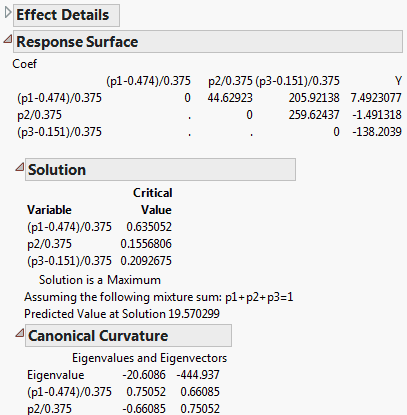
The Response Surface Solution report (Mixture Response Surface Analysis) shows that a maximum predicted value of 19.570299 occurs at point (0.63505, 0.15568, 0.20927).
|
1.
|
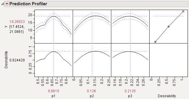
If the profiler is not visible, click the red triangle in the Response Y title bar and select Factor Profiling > Profiler. You should see the initial profiler shown in Initial Prediction Profiler.
|
Note: The axes of prediction profiler traces range from the upper and lower bounds of the factors, p1, p2, and p3, entered to create the design and the design table. When you experiment moving a variable trace, you see the other traces move such that their ratio is preserved. As a result, when the limit of a variable is reached, it cannot move further and only the third variable changes.
|
2.
|
To limit the visible profile curves to bounds that use all three variables, select Profile at Boundary > Stop at Boundaries from Prediction Profiler red triangle menu.
|
|
3.
|
If needed, select the Desirability Functions command to display the desirability function showing to the right of the prediction profile plots in Maximum Desirability in Profiler for Mixture Analysis Example.
|
|
4.
|
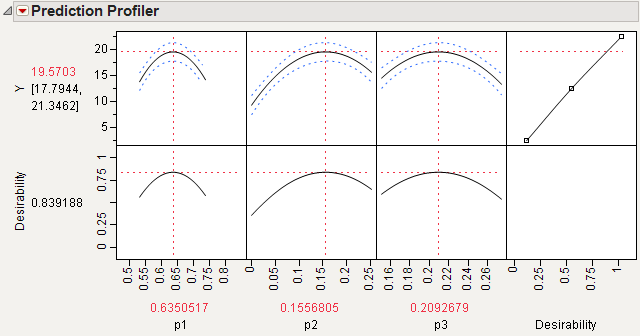
Select Maximize Desirability from the Prediction Profiler menu to see the best factor settings.
|
The profiler in Maximum Desirability in Profiler for Mixture Analysis Example, displays optimal settings (rounded) of 0.6350 for p1, 0.1557 for p2, and 0.2093 for p3, which give an estimated response of 19.5703.
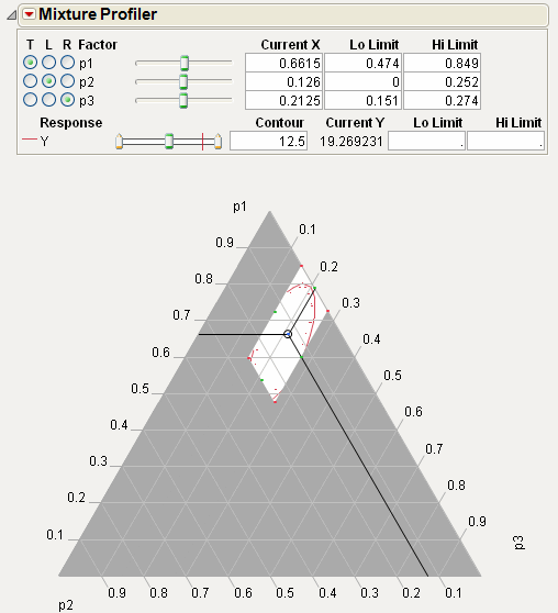
The Fit Model report also has a Mixture Profiler that is useful for visualizing and optimizing response surfaces from mixture experiments.
Select Factor Profiling > Mixture Profiler from Response Y red triangle menu to see the mixture profiler for the plasticizer data, shown in Mixture Profiler for Plasticizer Example.
|
1.
|
Choose Graph > Ternary Plot.
|
|
2.
|
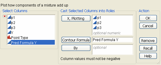
Specify plot variables (p1, p2, and p3) and click X, Plotting, as shown in Ternary Plot Launch Window.
|
|
3.
|
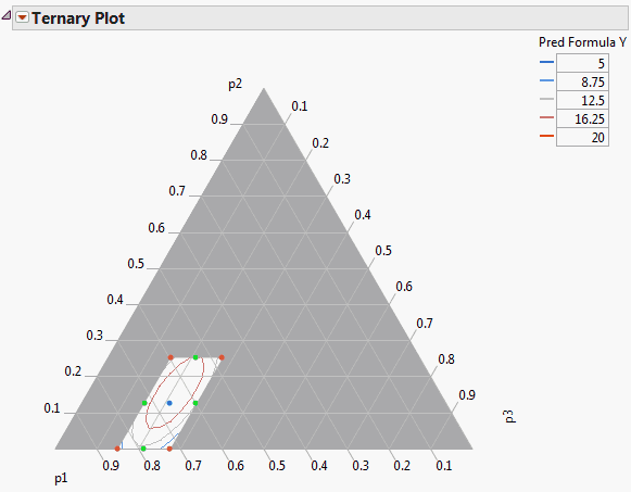
To identify the contour variable (the prediction equation), select Pred Formula Y and click the Contour Formula button. The contour variable must have a prediction formula to form the contour lines, as shown by the ternary plots at the bottom in Ternary Plot of a Mixture Response Surface. If there is no prediction formula, the ternary plot only shows points.
|
|
4.
|
By default, the ternary plot shows contour lines only. Add a fill by selecting Contour Fill from the Ternary Plot red triangle menu and then selecting Fill Above or Fill Below.
