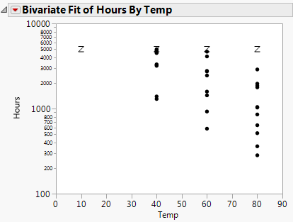
In the Devalt.jmp data, units are stressed by heating, in order to make them fail soon enough to obtain enough failures to fit the distribution.
|
1.
|
|
2.
|
Select Analyze > Fit Y by X.
|
|
3.
|
|
4.
|
|
5.
|
Click OK.
|
|
6.
|
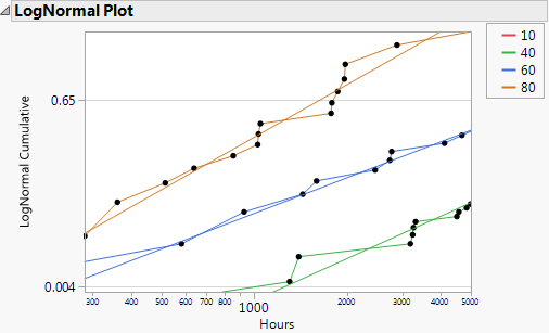
Select Analyze > Reliability and Survival > Survival.
|
|
7.
|
|
8.
|
|
9.
|
|
10.
|
|
11.
|
Click OK.
|
|
12.
|
|
13.
|
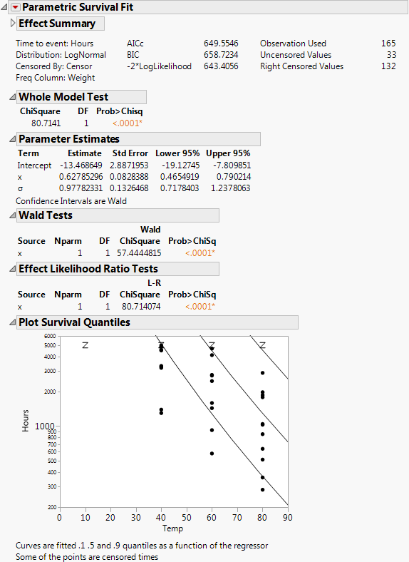
Select Analyze > Reliability and Survival > Fit Parametric Survival.
|
|
14.
|
|
15.
|
|
16.
|
|
17.
|
|
18.
|
|
19.
|
Click Run.
|
|
‒
|
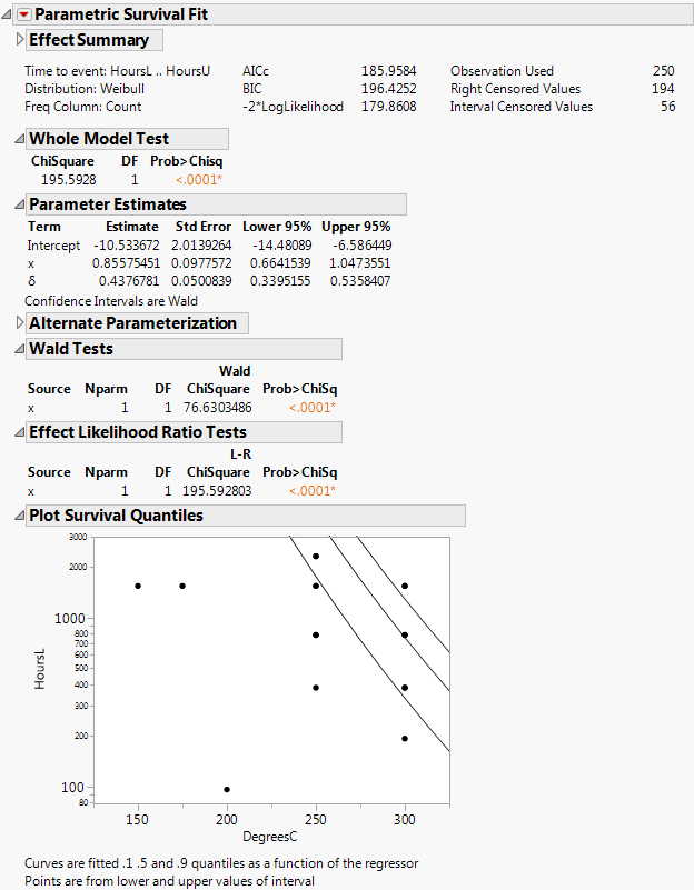
If the regressor column has a formula in terms of one other column, as in this case, the plot is done with respect to the inner column. In this case, the regressor was the column x, but the plot is done with respect to Temp, of which x is a function.
|
|
20.
|
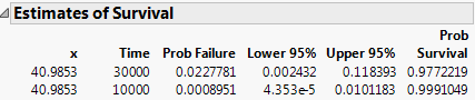
From the red triangle menu, select Estimate Survival Probability.
|
|
21.
|
Enter the values shown in Estimating Survival Probabilities into the Dialog to Estimate Survival.
|
|
22.
|
Click Go.
|
The ICdevice02.jmp data shows failures that were found to have happened between inspection intervals. The model uses two y-variables, containing the upper and lower bounds on the failure times. Right-censored times are shown with missing upper bounds.
|
1.
|
|
2.
|
Select Analyze > Reliability and Survival > Fit Parametric Survival.
|
|
3.
|
|
4.
|
|
5.
|
|
6.
|
Click Run.
|
ICDevice Output
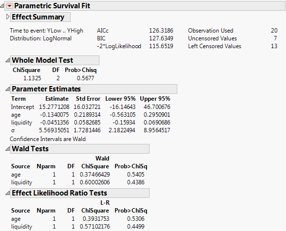
Note the following about the Tobit2.jmp data table:
|
•
|
The response variable is a measure of the durability of a product and cannot be less than zero (Durable, is left-censored at zero).
|
|
•
|
Age and Liquidity are independent variables.
|
|
•
|
The table also includes the model and tobit loss function. The model in residual form is durable-(b0+b1*age+b2*liquidity). To see the formula associated with Tobit Loss, right-click on the column and select Formula.
|
|
1.
|
|
2.
|
|
3.
|
|
4.
|
|
5.
|
Click OK.
|
|
6.
|
Click Go.
|
|
7.
|
Click Confidence Limits.
|
|
1.
|
|
2.
|
Select Analyze > Reliability and Survival > Fit Parametric Survival.
|
|
3.
|
|
4.
|
|
5.
|
|
6.
|
Click Run.
|
In this example, models are fit to the survival time using the Weibull, lognormal, and exponential distributions. Model fits include a simple survival model containing only two regressors, a more complex model with all the regressors and some covariates, and the creation of dummy variables for the covariate Cell Type to be included in the full model.
|
1.
|
The first model and all the loss functions have already been created as formulas in the data table. The Model column has the following formula:
|
2.
|
Select Analyze >Modeling > Nonlinear.
|
|
3.
|
|
4.
|
Click OK.
|
|
5.
|
Click Go.
|
|
6.
|
Click Save Estimates.
|
|
7.
|
Select Analyze >Modeling > Nonlinear again.
|
|
8.
|
|
9.
|
|
10.
|
Click OK.
|
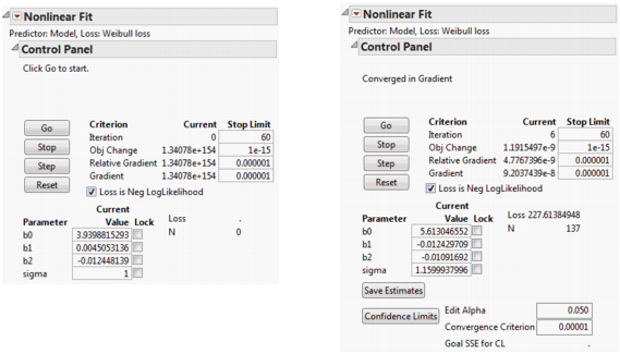
The Nonlinear Fit Control Panel on the left in Nonlinear Model with Custom Loss Function appears. There is now the additional parameter called sigma in the loss function. Because it is in the denominator of a fraction, a starting value of 1 is reasonable for sigma. When using any loss function other than the default, the Loss is Neg LogLikelihood box on the Control Panel is checked by default.
|
11.
|
Click Go.
|
|
12.
|
(Optional) Click Confidence Limits to show lower and upper 95% confidence limits for the parameters in the Solution table.
|
|
13.
|
(Optional) From the red triangle menu next to Nonlinear Fit, select Revert to Original Parameters.
|
The Loss Function Templates folder has templates with formulas for exponential, extreme value, loglogistic, lognormal, normal, and one-and two-parameter Weibull loss functions. To use these loss functions, copy your time and censor values into the Time and censor columns of the loss function template. To run the model, select Nonlinear and assign the loss column as the Loss variable. Because both the response model and the censor status are included in the loss function and there are no other effects, you do not need a prediction column (model variable).
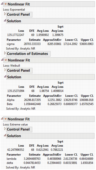
The Fan.jmp data table can be used to illustrate the Exponential, Weibull, and Extreme value loss functions discussed in Nelson (1982). The data are from a study of 70 diesel fans that accumulated a total of 344,440 hours in service. The fans were placed in service at different times. The response is failure time of the fans or run time, if censored.
Tip: To view the formulas for the loss functions, in the Fan.jmp data table, right-click the Exponential, Weibull, and Extreme value columns and select Formula.
|
1.
|
|
2.
|
|
3.
|
|
4.
|
Click OK.
|
|
5.
|
Make sure that the Loss is Neg LogLikelihood check box is selected.
|
|
6.
|
Click Go.
|
|
7.
|
Click Confidence Limits.
|
|
8.
|
The Locomotive.jmp data can be used to illustrate a lognormal loss. The lognormal distribution is useful when the range of the data is several powers of e.
Tip: To view the formula for the loss function, in the Locomotive.jmp data table, right-click on the logNormal column and select Formula.
The lognormal loss function can be very sensitive to starting values for its parameters. Because the lognormal distribution is similar to the normal distribution, you can create a new variable that is the natural log of Time and use Distribution to find the mean and standard deviation of this column. Then, use those values as starting values for the Nonlinear platform. In this example, the mean of the natural log of Time is 4.72 and the standard deviation is 0.35.
|
1.
|
|
2.
|
|
3.
|
|
4.
|
Click OK.
|
|
5.
|
Click Go.
|
|
6.
|
Click Confidence Limits.
|
The maximum likelihood estimates of the lognormal parameters are 5.11692 for Mu and 0.7055 for Sigma (in natural logs). The corresponding estimate of the median of the lognormal distribution is the antilog of 5.11692 (e5.11692), which is approximately 167. This represents the typical life for a locomotive engine.