This example tests for practical differences using the Probe.jmp sample data table.
|
1.
|
|
2.
|
Select Analyze > Modeling > Response Screening.
|
|
3.
|
|
4.
|
|
6.
|
Click OK.
|
|
7.
|
From the Response Screening report’s red triangle menu, select Save Compare Means.
|
Compare Means Table, Partial View shows a portion of the data table. For each response in Y, the corresponding row gives information about tests of the New and the Old levels of Process.
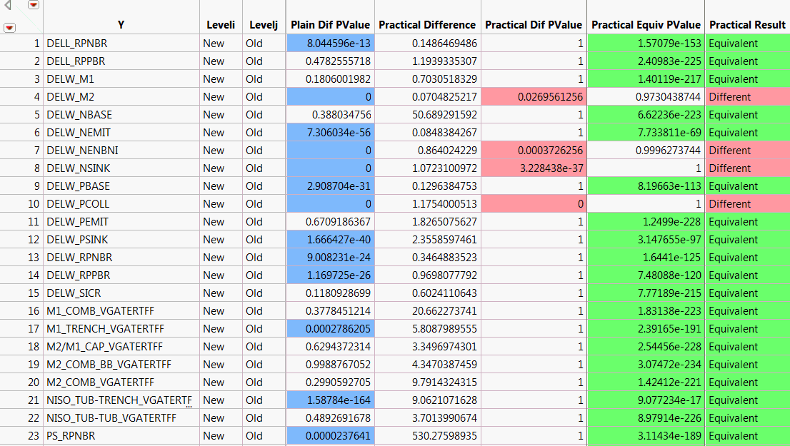
Because specification limits are not saved as column properties in Probe.jmp, JMP calculates a value of the practical difference for each response. The practical difference of 0.15 that you specified is multiplied by an estimate of the 6σ range of the response. This value is used in testing for practical difference and equivalence. It is shown in the Practical Difference column.
The Plain Difference column shows responses whose p-values indicate significance. The Practical Diff PValue and Practical Equiv PValue columns give the p-values for tests of practical difference and practical equivalence. Note that many columns show statistically significant differences, but do not show practically significant differences.
|
8.
|
Display the Compare Means data table and select Analyze > Distribution.
|
|
9.
|
|
10.
|
Click OK.
|
Distribution of Practical Significance Results shows the distribution of results for practical significance. Only 37 tests are different, as determined by testing for the specified practical difference. For 5 of the responses, the tests were inconclusive. You cannot tell whether the responses result in a practical difference across Process.
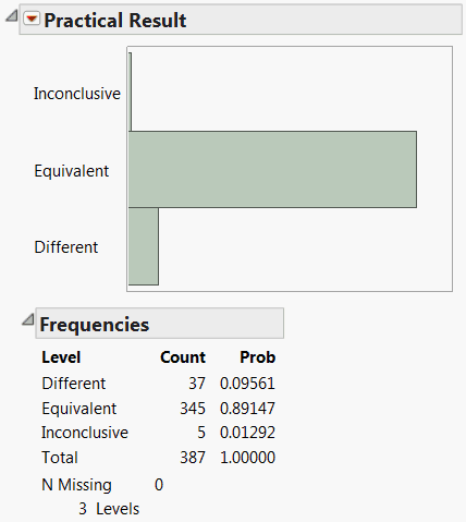
The 37 responses can be selected for further study by clicking on the corresponding bar in the plot.
When data sets have a large number of observations, p-values can be very small. LogWorth values provide a useful way to study p-values graphically in these cases. But sometimes p-values are so small that the LogWorth scale is distorted by huge values.
|
1.
|
|
2.
|
Select Analyze > Modeling > Response Screening.
|
|
3.
|
|
4.
|
|
5.
|
Select the Robust check box.
|
|
6.
|
Click OK.
|
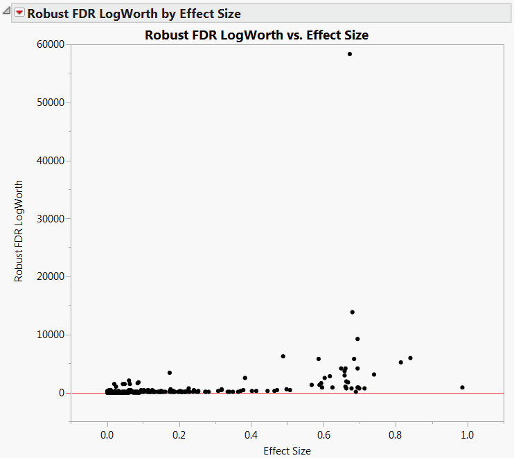
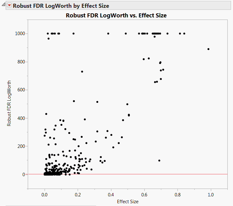
The detail in the plot is hard to see, because of the huge Robust FDR LogWorth value of about 58,000 (Robust FDR LogWorth vs. Effect Size, MaxLogWorth Not Set). To ensure that your graphs show sufficient detail, you can set a maximum value of the LogWorth.
|
10.
|
Click OK.
|
|
1.
|
Open the Drosophila Aging.jmp table.
|
|
2.
|
Select Analyze > Modeling > Response Screening.
|
|
3.
|
Select all of the continuous columns and click Y, Response.
|
|
4.
|
|
5.
|
Check Robust.
|
|
6.
|
Click OK.
|
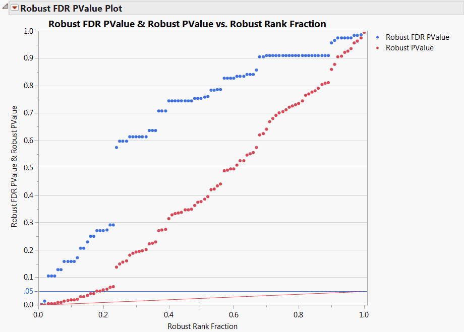
The Robust FDR PValue Plot is shown in Robust FDR PValue Plot for Drosophila Data. Note that a number of tests are significant using the unadjusted robust p-values, as indicated by the red points that are less than 0.05. However, only two tests are significant according to the robust FDR p-values.
|
9.
|
In the PValues data table, select Rows > Label/Unlabel.
|
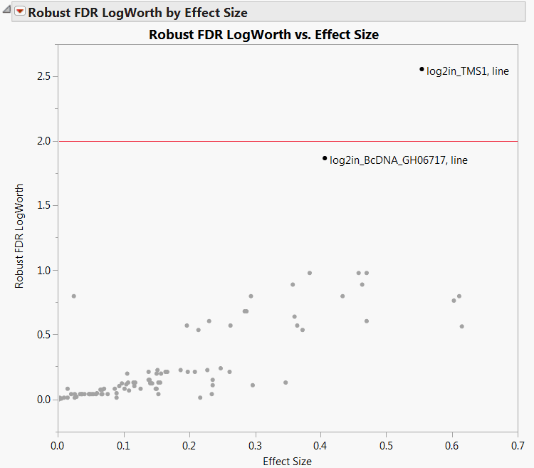
The plot shown in Robust LogWorth by Effect Size for Drosophila Data appears. Points above the red line at 2 have significance levels below 0.01. A horizontal line at about 1.3 corresponds to a 0.05 significance level.
The plot shown in Robust LogWorth by LogWorth for Drosophila Data. If the robust test for a response were identical to the usual test, its corresponding point would fall on the diagonal line in Robust LogWorth by LogWorth for Drosophila Data. The circled point in the plot does not fall near the line, because it has a Robust LogWorth value that exceeds its LogWorth value.
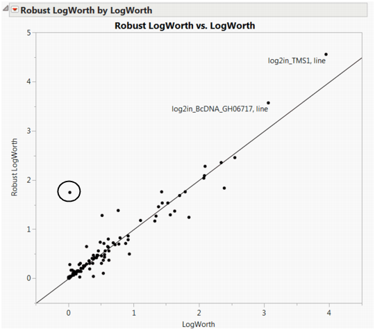
Note that the response, log2in_CG8237 has PValue 0.9568 and Robust PValue 0.0176.
|
13.
|
In the Response screening report, select Fit Selected Items from the red triangle menu.
|
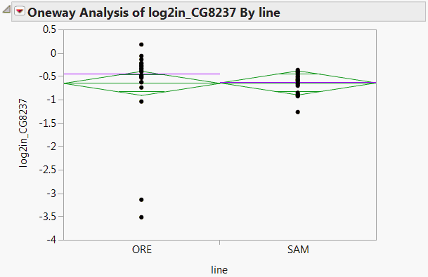
A Fit Selected Items report is displayed containing a Oneway Analysis for the response log2in_CG8237. The plot shows two outliers for the ORE line (Oneway Analysis for log2in_CG8237). These outliers indicate why the robust test and the usual test give disparate results. The outliers inflate the error variance for the non-robust test, which makes it more difficult to see a significant effect. In contrast, the robust fit down-weights these outliers, thereby reducing their contribution to the error variance.
|
1.
|
Open the Drosophila Aging.jmp table.
|
|
2.
|
Select Analyze > Fit Model.
|
|
4.
|
|
5.
|
|
6.
|
Select Response Screening from the Personality list.
|
|
7.
|
Click Run.
|
|
8.
|
Run the FDR LogWorth by Rank Fraction script in the PValues data table.
|
|
9.
|
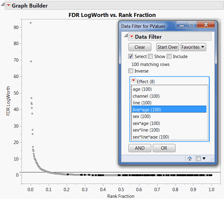
Select Rows > Data Filter.
|
|
10.
|
Keep in mind that values of LogWorth that exceed 2 are significant at the 0.01 level. The Data Filter helps you see that, with the exception of sex and channel, the model effects are rarely significant at the 0.01 level. FDR LogWorth vs Rank Fraction Plot with line*age Tests Selected shows a reference line at 2. The points for tests of the line*age interaction effect are selected. None of these are significant at the 0.01 level.