where K is a constant equal to the 0.75 quantile of a chi-square distribution with the degrees of freedom equal to the number of columns in the data table, and
where yi = the response for the ith observation, μ = the current estimate of the mean vector, S2 = current estimate of the covariance matrix, and T = the transpose matrix operation. The final step is a bias reduction of the variance matrix.
The Pearson product-moment correlation coefficient measures the strength of the linear relationship between two variables. For response variables X and Y, it is denoted as r and computed as

Spearman’s ρ (rho) Coefficients
Spearman’s ρ correlation coefficient is computed on the ranks of the data using the formula for the Pearson’s correlation previously described.
Kendall’s τb coefficients are based on the number of concordant and discordant pairs. A pair of rows for two variables is concordant if they agree in which variable is greater. Otherwise they are discordant, or tied.


|
•
|
The ti (the ui) are the number of tied x (respectively y) values in the ith group of tied x (respectively y) values.
|
|
•
|
The n is the number of observations.
|
|
•
|
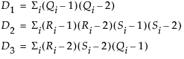
The formula for Hoeffding’s D (1948) is

|
•
|
|
•
|
The Qi (sometimes called bivariate ranks) are one plus the number of points that have both x and y values less than the ith points.
|
|
•
|
A point that is tied on its x value or y value, but not on both, contributes 1/2 to Qi if the other value is less than the corresponding value for the ith point. A point tied on both x and y contributes 1/4 to Qi.
|
When there are no ties among observations, the D statistic has values between –0.5 and 1, with 1 indicating complete dependence. If a weight variable is specified, it is ignored.
The inverse correlation matrix provides useful multivariate information. The diagonal elements of the inverse correlation matrix, sometimes called the variance inflation factors (VIF), are a function of how closely the variable is a linear function of the other variables. Specifically, if the correlation matrix is denoted R and the inverse correlation matrix is denoted R-1, the diagonal element is denoted rii and is computed as

where Ri2 is the coefficient of variation from the model regressing the ith explanatory variable on the other explanatory variables. Thus, a large rii indicates that the ith variable is highly correlated with any number of the other variables.
The Mahalanobis distance takes into account the correlation structure of the data and the individual scales. For each value, the Mahalanobis distance is denoted Mi and is computed as
Y is the row of means
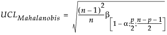
n = number of observations
p = number of variables (columns)

n = number of observations
p = number of variables (columns)

T2 Distance Measures

n = number of observations
p = number of variables (columns)
Cronbach’s α is defined as
k = the number of items in the scale
c = the average covariance between items
v = the average variance between items
r = the average correlation between items
The larger the overall α coefficient, the more confident you can feel that your items contribute to a reliable scale or test. The coefficient can approach 1.0 if you have many highly correlated items.