The Estimates menu provides additional detail about model parameters. To better understand estimates, you might want to review JMP’s approach to coding nominal and ordinal effects. See Details of Custom Test Example, Nominal Factors in Statistical Details, and Ordinal Factors in Statistical Details).
The Show Prediction Expression option shows the equation used to predict the response. Prediction Expression shows an example for the Drug.jmp sample data table. This expression is given as a typical JMP formula. For example, to predict the response for someone on Drug a with x = 10, you would calculate, with some rounding: –2.696 - 1.185 + 0.987(10) = 5.99.
|
1.
|
|
2.
|
Select Analyze > Fit Model.
|
|
3.
|
|
4.
|
|
5.
|
Click Run.
|
|
6.
|
From the red triangle menu next to Response y, select Estimates > Show Prediction Expression. The report in Prediction Expression appears.
|
The Sorted Estimates option produces a version of the Parameter Estimates report that is useful in screening situations. If the design is not saturated, the Sorted Estimates report gives the information found in the Parameter Estimates report, but with the terms, other than the Intercept, sorted in decreasing order of significance (second report in Sorted Parameter Estimates). If the design is saturated, then Pseudo t tests are provided. These are based on Lenth’s pseudo standard error (Lenth, 1989). See Lenth’s PSE.
|
1.
|
|
2.
|
Select Analyze > Fit Model.
|
|
3.
|
|
4.
|
Make sure that 2 appears in the Degree box near the bottom of the window.
|
|
5.
|
|
6.
|
Click Run.
|
Note the following differences between the Parameter Estimates report and the Sorted Parameter Estimates report (both shown in Sorted Parameter Estimates):
|
•
|
The effects are sorted by the absolute value of the t ratio, showing the most significant effects at the top.
|
|
•
|
A bar chart shows the t ratio with vertical lines showing critical values for the 0.05 significance level.
|
Screening experiments often involve fully saturated models, where there are not enough degrees of freedom to estimate error. In these cases, the Sorted Estimates report (Sorted Parameter Estimates) gives relative standard errors and constructs t ratios and p-values using Lenth’s pseudo standard error (PSE). These quantities are labeled with Pseudo in their names. See Lenth’s PSE and Pseudo t-Ratios.
The parameter estimates are presented in sorted order, with smallest p-values listed first.
A t ratio for the estimate, computed using pseudo standard error. The value of Lenth PSE is shown in a note at the bottom of the report.
A p-value computed using an error degrees of freedom value (DFE) of m/3, where m is the number of parameters other than the intercept. The value of DFE is shown in a note at the bottom of the report.
Lenth’s pseudo standard error (PSE) is an estimate of residual error due to Lenth (1989). It is based on the principle of effect sparsity: in a screening experiment, relatively few effects are active. The inactive effects represent random noise and form the basis for Lenth’s estimate.
|
2.
|
When relative standard errors are equal, Lenth’s PSE is shown in a note at the bottom of the report. The Pseudo t-Ratio is calculated as follows:
When relative standard errors are not equal, the TScale Lenth PSE is computed. This value is the PSE of the estimates divided by their relative standard errors. The Pseudo t-Ratio is calculated as follows:
|
1.
|
|
2.
|
Select Analyze > Fit Model.
|
|
3.
|
|
4.
|
|
5.
|
|
6.
|
Click Run.
|
The Sorted Parameter Estimates report appears (Sorted Parameter Estimates Report for Saturated Model). Note that Lenth’s PSE and the degrees of freedom used are given at the bottom of the report. The report indicates that, based on their Pseudo p-Values, the effects Ct, Ct*T, T*Cn, T, and Cn are highly significant.
In dealing with parameter estimates, you must understand how JMP codes nominal and ordinal columns. For details about how nominal columns are coded, see Details of Custom Test Example. For complete details about how ordinal columns are coded and modeled, see Nominal Factors and Ordinal Factors.
Use the Expanded Estimates option when there are nominal terms in the model and you want to see details for the full set of estimates. The Expanded Estimates option provides the estimates, their standard errors, t ratios, and p-values.
|
1.
|
|
2.
|
Select Analyze > Fit Model.
|
|
3.
|
|
4.
|
|
5.
|
Click Run.
|
|
6.
|
From the red triangle menu next to Response y, select Estimates > Expanded Estimates.
|
The Expanded Estimates report, along with the Parameter Estimates report, is shown in Comparison of Parameter Estimates and Expanded Estimates. Note that an estimate for the term Drug[f] appears in the Expanded Estimates report. The null hypothesis for the test is that the mean for the Drug f group does not differ from the overall mean. The test for Drug[f] is significant at the 0.05 level, suggesting that the mean response for the Drug f group differs from the overall response. See Interpretation of Tests for Expanded Estimates for more details.
Suppose that your model consists of a single nominal factor that has n levels. That factor is represented by n-1 indicator variables, one for each of n-1 levels. The parameter estimate corresponding to any one of these n-1 indicator variables is the difference between the mean response for that level and the average response across all levels. This representation is due to the way that JMP codes nominal variables (see Details of Custom Test Example). The parameter estimate is often interpreted as the effect of that level.
For example, in the Cholesterol.jmp sample data table, consider the single factor treatment and the response June PM. The parameter estimate associated with the term, or indicator variable, treatment[A] is the difference between the mean of June PM for treatment A and the overall mean of June PM.
The effects across all levels of a nominal variable are constrained to sum to zero. Consider the effect of the last level in the level ordering, namely, the level that is coded with –1s. The effect of this level is the negative of the sum of the effects across the other n-1 levels. It follows that the effect of the last level is the negative of the sum of the parameter estimates across the other n-1 levels.
In the Drug.jmp report shown in Comparison of Parameter Estimates and Expanded Estimates, the estimates for the terms associated with Drug are based on a model that includes the covariate x.
|
•
|
The estimate for Drug[a] is the difference between the least squares mean for Drug a and the overall mean of y.
|
|
•
|
The t test for Drug [f] presented in the Expanded Estimates report tests whether the response for the Drug f group differs from the overall mean response.
|
|
•
|
If nominal factors are involved in high-degree interactions, the Expanded Estimates report can be lengthy. For example, a five-way interaction of two-level nominal factors produces only one parameter estimate but has 25 = 32 expanded effects, which are all identical up to sign changes.
|
This option displays parameter estimates for the model where nominal and ordinal columns have been coded using the SAS GLM parameterization. The SAS GLM and JMP coding schemes are described in The Factor Models in Statistical Details.
To create the report in Indicator Parameterization Estimates, follow the steps in Example of an Expanded Estimates Report. But instead of selecting Expanded Estimates, select Indicator Parameterization Estimates.
The Sequential Tests report shows sums of squares and tests as effects are added to the model sequentially. The order of entry is defined by the order of effects as they appear in the Fit Model launch window’s Construct Model Effects list. The report in Sequential Tests Report is for the Drug.jmp sample data table.
The sums of squares that form the basis for sequential tests are also called Type I Sums of Squares. They are computed by fitting models in steps following the specified entry order of effects. Consider a specific effect. Compute the model sum of squares for a model containing all effects entered prior to that effect. Then compute the model sum of squares for a model containing those effects and the specified effect. The sequential sum of squares for the specified effect is the increase in the model sum of squares.
Refer to Sequential Tests Report, showing sequential sums of squares for the Drug.jmp sample data table. In the Fit Model launch window, Drug was entered first, followed by x. A model consisting only of Drug has model sum of squares equal to 293.6. When x is added to the model, the model sum of squares becomes 871.4974. The increase of 577.8974 is the sequential sum of squares for x.
The tests shown in the Sequential (Type 1) Tests report are F tests based on sequential sums of squares, also called Type I Tests. The F Ratio tests the specified effect, where the model contains only that effect and the effects listed above it in the Source column.
The tests given in the Parameter Estimates and Effect Tests reports are based on Type III Sums of Squares. Here the sum of squares for an effect is the extra sum of squares explained by the effect after all other effects have been entered in the model.
To test one or more custom hypotheses involving any model parameters, select Custom Test from the Estimates menu. In this window, you can specify one or more linear functions, or contrasts, of the model parameters.
The results include individual tests for each contrast and a joint test for all contrasts. See Custom Test Specification Window for Three Contrasts. The report for the individual contrasts gives the estimated value of the specified linear function of the parameters and its standard error. A t ratio, its p-value, and the associated sum of squares are also provided. Below the individual contrast results, the joint test for all contrasts gives the sum of squares, the numerator degrees of freedom, the F ratio, and its p-value.
Click the Done button to perform the tests. The report changes to show the test statistic value, the standard error, and other statistics for each test column. The joint F test for all columns is given in a box at the bottom of the report.
Provides a power analysis for the joint test. This option is available only after the test has been conducted. For details, see Parameter Power.
Custom Test Specification Window for Three Contrasts shows an example of the specification window with three contrasts, using the Cholesterol.jmp sample data table. Note that the constant is set to zero for all three tests. The report for these tests is shown in Custom Test Report Showing Tests for Three Contrasts.
The Cholesterol.jmp sample data table gives repeated measures on 20 patients at six time periods. Four treatment groups are studied. Typically, this data should be properly analyzed using all repeated measures as responses. This example considers only the response for June PM.
|
1.
|
|
2.
|
Select Analyze > Fit Model.
|
|
3.
|
|
4.
|
|
5.
|
Click Run.
|
|
6.
|
|
7.
|
In the Custom Test specification window, click Add Column twice to create three columns.
|
|
8.
|
To see how to obtain these values, particularly those in the third column, see Base Model for Nominal Responses in Statistical Details.
|
9.
|
Click Done.
|
The results shown in Custom Test Report Showing Tests for Three Contrasts indicate that all three hypotheses are individually, as well as jointly, significant.
To see how to obtain these values, particularly those in the third column, see Base Model for Nominal Responses in Statistical Details.
Use this option to obtain tests and confidence levels that compare means defined by levels of your model effects. The goal when making multiple comparisons is to determine if group means differ, while controlling the probability of reaching an incorrect conclusion. The Multiple Comparisons option lets you compare group means with an overall average mean (Analysis of Means) and with a control group mean. You can also conduct pairwise comparisons using either Tukey HSD or Student’s t. To identify pairwise differences that are of practical importance, you can perform equivalence tests.
The Student’s t method only controls the error rate for an individual comparison. As such, it is not a true multiple comparison procedure. All other methods provided control the overall error rate for all comparisons of interest. Each of these methods uses a multiple comparison adjustment in calculating p-values and confidence limits.
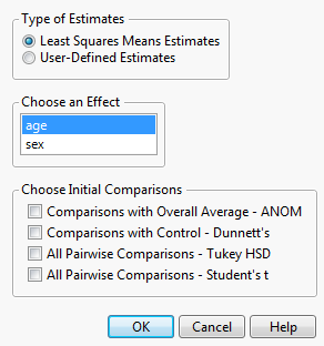
An example of the control window for the Multiple Comparisons option is shown in Launch Window for Least Squares Means Estimates. This example is based on the Big Class.jmp data table, with weight as Y and age, sex, and height as model effects. Two classes of estimates are available for comparisons: Least Squares Means Estimates and User-Defined Estimates.
This option compares least squares means and is available only if there are nominal or ordinal effects in the model. Recall that least squares means are means computed at some neutral value of the other effects in the model. (For a definition of least squares means, see LSMeans Table.) You must select the effect of interest. In Launch Window for Least Squares Means Estimates, Least Squares Means Estimates for age are specified.
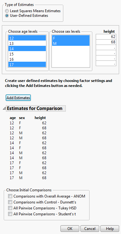
The specification of User-Defined Estimates is illustrated in Launch Window for User-Defined Estimates. Three levels of age and both levels of sex have been selected. Also, two values of height have been manually entered. The Add Estimates button has been clicked, resulting in the listing of all possible combinations of the specified levels. At this point, you can specify more estimates and click the Estimates button again to add them to the list of Estimates for Comparison.
Note: In this section, we will use the term mean to refer to either estimates of least squares means or user-defined estimates.
Shows the t ratio for the significance test.
Gives the p-value for the significance test.
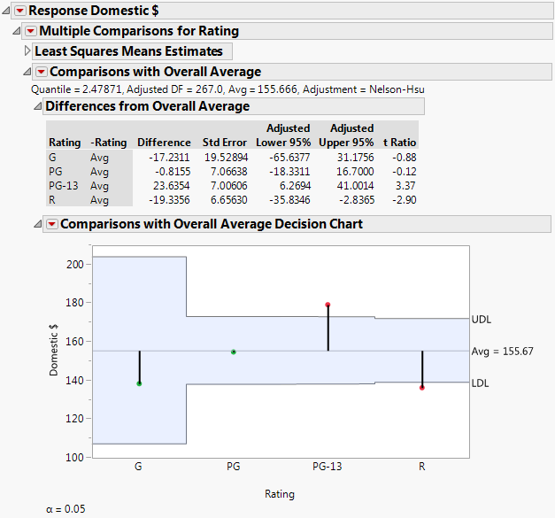
This option compares the means for the specified levels specified to the overall mean for these levels. It displays a table showing confidence intervals for differences from the overall mean and a chart showing decision limits. The method used to make the comparisons is called analysis of means (ANOM) (Nelson, et al., 2005). ANOM is a multiple comparison procedure that controls the joint error rate for all pairwise comparisons to the overall mean. See Comparisons with Overall Average for Ratings for a report based on the Movies.jmp sample data table.
The value of Nelson’s h statistic used in constructing the decision limits.
Specifically, the average least squares mean is a weighted average with weights inversely proportional to the diagonal entries of the matrix  . Here L is the matrix of coefficients used to compute the group least squares means. For a technical definition of least squares means and the average least squares mean, see the GLM Procedure section in the SAS/STAT 9.3 User’s Guide. Search for “Construction of Least Squares Means”.
For user-defined estimates, the average mean is defined similarly. However, in this case, L is the matrix of coefficients used to define the estimates.
|
‒
|
Nelson: Provides exact critical values and p-values. Used whenever possible, in particular, when the estimates are uncorrelated.
|
|
‒
|
Nelson-Hsu: Provides approximate critical values and p-values based on Hsu’s factor analytical approximation is used (Hsu, 1992). Used when exact values can not be obtained.
|
For technical details, see the GLM Procedure section in the SAS/STAT 9.3 User’s Guide. Search for “Approximate and Simulation-Based Methods”.
Adds columns giving t ratios (t Ratio) and p-values (Prob>|t|) to the Comparisons with Overall Average report. Note that computing exact critical values and p-values for unbalanced designs requires complex integration and can be computationally challenging. When calculations for such a quantile fail, the Sidak quantile is computed but p-values are not available.
Consider the Movies.jmp sample data table. You are interested in whether any of the four Rating categories are unusual in that their mean Domestic $ revenues differ from the overall average revenue. You specify a model with Domestic $ as the response and Type, Rating, and Year as model effects.
|
1.
|
|
2.
|
Select Analyze > Fit Model.
|
|
3.
|
|
4.
|
|
5.
|
Click Run.
|
|
6.
|
|
7.
|
|
8.
|
In the Choose Initial Comparisons list, select Comparisons with Overall Average.
|
|
9.
|
Click OK.
|
|
10.
|
From the Comparisons with Overall Average red triangle menu, select Calculate P-Values.
|
The results shown in Comparisons with Overall Average for Ratings indicate that the least squares means for movies with a Rating of PG-13 and R differ significantly from the overall average in terms of Domestic $.
|
‒
|
Dunnett: Provides exact critical values and p-values. Used whenever possible, in particular, when the estimates are uncorrelated.
|
|
‒
|
Dunnett-Hsu: Provides approximate critical values and p-values based on Hsu’s factor analytical approximation (Hsu, 1992). Used when exact values can not be obtained.
|
For technical details, see the GLM Procedure section in the SAS/STAT 9.3 User’s Guide. Search for “Approximate and Simulation-Based Methods”.
For each comparison of a group mean to the control mean, this report provides the following details:
Adds columns giving t ratios (t Ratio) and p-values (Prob>|t|) to the Comparisons with Control report. Note that computing exact critical values and p-values for unbalanced designs requires complex integration and can be computationally challenging. When calculations for such a quantile fail, the Sidak quantile is computed but p-values are not available.
The All Pairwise Comparisons option shows either a Tukey HSD All Pairwise Comparisons or Student’s t All Pairwise Comparisons report (Hsu, 1996 and Westfall et al., 2011). Tukey HSD comparisons are constructed so that the significance level applies jointly to all pairwise comparisons. In contrast, for Student’s t comparisons, the significance level applies to each individual comparison. When making several pairwise comparisons using Student’s t tests, the risk that one of the comparisons incorrectly signals a difference can well exceed the stated significance level.
The critical value for the test. Note that, for Tukey HSD, the quantile is  , where q is the appropriate percentage point of the studentized range statistic.
|
‒
|
Tukey: Provides exact critical values and p-values. Used when the means are uncorrelated and have equal variances, or when the design is variance-balanced.
|
|
‒
|
Tukey-Kramer: Provides approximate critical values and p-values. Used when exact values can not be obtained.
|
For technical details, see the GLM Procedure section in the SAS/STAT 9.3 User’s Guide. Search for “Approximate and Simulation-Based Methods”.
Both Tukey HSD and Student’s t compare all pairs of levels. For each pairwise comparison, the All Pairwise Differences report shows:
|
•
|
t Ratio - the t ratio for the test of whether the difference is zero
|
|
•
|
Prob > |t| - the p-value for the test
|
This plot, sometimes called a diffogram or a mean-mean scatterplot, displays the confidence intervals for all means pairwise differences. (See All Pairwise Comparisons Scatterplot for User-Defined Comparisons for an example.) Colors indicate which differences are significant.
Use this option to conduct one or more equivalence tests. Equivalence tests are useful when you want to detect differences that are of practical interest. You are asked to specify a threshold difference for group means for which smaller differences are considered practically equivalent. In other words, if two group means differ by this amount or less, you are willing to consider them equivalent.
Once you have specified this value, the Equivalence Tests report appears. The bounds that you have specified are given at the top of the report. The report consists of a table giving the equivalence tests and a scatterplot that displays them. The equivalence tests and confidence intervals are based on Tukey HSD or Student’s t critical values, corresponding to the option that you selected.
The Two One-Sided Tests (TOST) method is used to test for a practical difference between the means (Schuirmann, 1987). Two one-sided pooled-variance t tests are constructed for the null hypotheses that the true difference exceeds the threshold values. If both tests reject, the difference in the means does not statistically exceed either threshold value. Therefore, the groups are considered practically equivalent. If only one or neither test rejects, then the groups might not be practically equivalent.
|
•
|
Lower Bound t Ratio, Upper Bound t Ratio - the lower and upper bound t ratios for the two one-sided pooled-variance significance tests
|
|
•
|
Lower Bound p-Value, Upper Bound p-value - p-values corresponding to the lower and upper bound t ratios
|
Using colors, this scatterplot indicates which means are practically equivalent and which are not as determined by the equivalence test. (See Equivalence Tests Scatterplot.)
Consider the Movies.jmp sample data table. You are interested in Domestic $ differences for action and drama movies across two Rating categories, PG-13 and R, in the year 1998.
|
1.
|
|
2.
|
Select Analyze > Fit Model.
|
|
3.
|
|
4.
|
|
5.
|
Click Run.
|
|
6.
|
|
7.
|
From the Type of Estimates list, click User-Defined Estimates.
|
|
10.
|
In the list entitled Year, enter the year 1998.
|
|
11.
|
Click Add Estimates. Note that all possible combinations of the levels you specified are now displayed beneath the Add Estimates button.
|
|
12.
|
In the Choose Initial Comparisons list, select All Pairwise Comparisons - Tukey HSD.
|
|
13.
|
Click OK.
|
The All Pairwise Differences report indicates that three of the six pairwise comparisons are significant. The All Pairwise Comparisons Scatterplot, shown in All Pairwise Comparisons Scatterplot for User-Defined Comparisons, shows the confidence intervals for these comparisons in red. Also shown is the tooltip for one of these intervals, indicating that the interval compares Action, Rating R movies to Drama, Rating PG-13 movies, and that the mean difference in Domestic $ is -53.58.
|
14.
|
|
16.
|
Click OK.
|
TOST tests are conducted to determine which movie categories are equivalent, given that you consider categories that differ by less than 50 in units of Domestic $ to be equivalent. The Equivalence Tests Scatterplot (Equivalence Tests Scatterplot) indicates that two pairs of movie categories can be considered equivalent.
|
1.
|
|
2.
|
Select Analyze > Fit Model.
|
|
3.
|
|
4.
|
Verify that 2 appears in the Degree box.
|
|
5.
|
|
6.
|
Click Run.
|
|
7.
|
From the red triangle next to Response weight, select Estimates > Joint Factor Tests.
|
Note that the test for age has 15 degrees of freedom. This test involves the five parameters for age, the five parameters for age*sex, and the five parameters for height*age. The null hypothesis for this test is that all 15 parameters are zero.
Inverse prediction occurs when you use a statistical model to infer the value of an explanatory variable, given a value of the response variable. Inverse prediction is sometimes referred to as calibration.
By selecting Inverse Prediction on the Estimates menu, you can estimate values of an independent variable, X, that correspond to specified values of the response (Inverse Prediction Specification for a Multiple Regression Model). In addition, you can specify values for other explanatory variables in the model (Inverse Prediction Specification for a Multiple Regression Model). The inverse prediction computation provides confidence limits for values of X that correspond to the specified response value. You can specify the response value to be the mean response or simply an individual response. For an example, see Example of Inverse Prediction.
The inverse prediction window shows the list of explanatory variables to the left. (See Inverse Prediction Specification for a Multiple Regression Model for an example.) Each continuous variable is initially set to its mean. Each nominal or ordinal variable is set to its lowest level (in terms of value ordering). You must remove the value for the variable that you want to predict, setting it to missing. Also, you must specify the values of the other variables for which you want your inverse prediction to hold (if these differ from the default settings). In the list to the right in the window, you can supply one or more response values of interest. For an example, see Example of Predicting a Single X Value with Multiple Model Effects.
Note: The confidence limits for inverse prediction can sometimes result in a one-sided or even an infinite interval. For technical details, see Inverse Prediction with Confidence Limits in Statistical Details.
In this example, you fit a regression model that predicts oxygen uptake from Runtime. Then you estimate the Runtime values that result in specified oxygen uptake values. There is only a single X, Runtime, so you start by using the Fit Y by X platform to obtain a visual approximation of the inverse prediction values.
|
1.
|
|
2.
|
Select Analyze > Fit Y by X.
|
|
3.
|
|
4.
|
|
5.
|
Click OK.
|
|
6.
|
From the red triangle menu, select Fit Line.
|
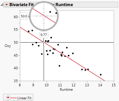
Use the crosshair tool as described below to approximate the Runtime value that results in a mean Oxy value of 50.
|
7.
|
Select Tools > Crosshairs.
|
|
8.
|
Click the Oxy axis at about 50 and then drag the cursor so that the crosshairs intersect with the prediction line.
|
Bivariate Fit for Fitness.jmp shows that a Runtime of about 9.77 gives an inverse prediction of about 50 for Oxy.
Bivariate Fit for Fitness.jmp
To obtain an exact prediction for Runtime, along with a confidence interval, use the Fit Model launch window as follows:
|
1.
|
|
2.
|
|
3.
|
|
4.
|
Click Run.
|
|
5.
|
From the red triangle menu next to Response Oxy, select Estimates > Inverse Prediction.
|
|
6.
|
|
7.
|
Click OK.
|
The Inverse Prediction report (Inverse Prediction Report) gives predicted Runtime values that correspond to each specified Oxy value. The report also shows upper and lower 95% confidence limits for these Runtime values, relative to obtaining the mean response.
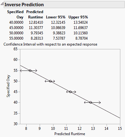
The exact predicted Runtime resulting in an Oxy value of 50 is 9.7935. This value is close to the approximate Runtime value of 9.77 found in the Bivariate Fit report shown in Bivariate Fit for Fitness.jmp. The Inverse Prediction report also gives a plot showing the linear relationship between Oxy and Runtime and the confidence intervals.
This example predicts the Runtime that results in oxygen uptake of 50 when RstPulse is 60. The Runtime is predicted for both males and females.
|
1.
|
|
2.
|
|
3.
|
|
4.
|
Click Run.
|
|
5.
|
From the red triangle menu next to Response Oxy, select Estimates > Inverse Prediction.
|
|
6.
|
Delete the value for Runtime, because you want to predict that value.
|
|
7.
|
|
8.
|
Replace the mean for RstPulse with 60.
|
|
9.
|
|
10.
|
Click OK.
|
The report, shown in Inverse Prediction Report for a Multiple Regression Model, gives the predicted values of Runtime for both females and males. The report also includes 95% confidence intervals for Runtime values that give a mean response of 50.
The plot shows the linear fits for females and males, given that RstPulse is 60. The two confidence intervals are shown in red and blue, respectively. Note that the intervals overlap, indicating that the true values of Runtime leading to an Oxy value of 50 might be identical for both males and females.
|
1.
|
|
2.
|
|
‒
|
Right-click on the column heading and select Column Info.
|
|
‒
|
Click OK.
|
|
3.
|
Select Analyze > Fit Model.
|
|
4.
|
|
5.
|
|
6.
|
Select Macros > Mixture Response Surface.
|
|
7.
|
Click Run.
|
|
8.
|
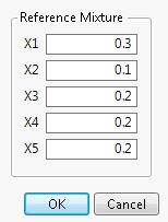
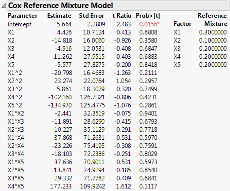
From the red triangle menu next to Response Y1, select Estimates > Cox Mixtures.
|
|
10.
|
Click OK.
|
The report (Cox Mixtures) shows the parameter estimates for the Cox mixture model, along with standard errors, and hypothesis tests. The reference mixture is displayed on the right.
The power of a statistical test is the probability that the test will be significant, if a difference actually exists. The power of the test indicates how likely your study is to declare a true effect to be significant. The Parameter Power option addresses retrospective power analysis.
Note: To ensure that your study includes sufficiently many observations to detect the required differences, use information about power when you design your experiment. This type of analysis is called prospective power analysis. Consider using the DOE platform to design your study. Both DOE > Sample Size and Power and DOE > Evaluate Design are useful for prospective power analysis. For an example of a prospective power analysis using standard least squares, see Prospective Power Analysis.
|
•
|
LSV0.05 is the least significant value. This number is the smallest absolute value of the estimate that would make this test significant at significance level 0.05. To be more specific, suppose that the number of observations, the mean square error and that the sum of squares and cross-products matrix for the design remain unchanged. Then, if the absolute value of the estimate had been less than LSV0.05, the Prob>|t| value would have exceeded 0.05. (For more details, see The Least Significant Value (LSV).)
|
|
•
|
LSN is the least significant number. This number is the number of observations that would make this test significant at significance level 0.05. Specifically, suppose that the estimate of the parameter, the mean square error, and the sum of squares and cross-products matrix for the design remain unchanged. Then, if the number of observations had been less than the LSN, the Prob>|t| value would have exceeded 0.05. (For more details, see The Least Significant Number (LSN).)
|
|
•
|
AdjPower0.05 is the adjusted power value. This number is an estimate of the probability that this test will be significant. Sample values from the current study are substituted for the parameter values typically used in a power calculation. The adjusted power calculation adjusts for bias that results from direct substitution of sample estimates into the formula for the non-centrality parameter (Wright and O’Brien, 1988). (For more details, see The Adjusted Power and Confidence Intervals.)
|
For further details about LSV, LSN, and adjusted power, see Power Analysis. For an example of a retrospective analysis, see Example of Retrospective Power Analysis.
For insight on the construction of this matrix, consider the typical least squares regression formulation. Here, the response (Y) is a linear function of predictors (x’s) plus error (ε):
Each row of the data table contains a response value and values for the p predictors. For each observation, the predictor values are considered fixed. However, the response value is considered to be a realization of a random variable.
Considering the values of the predictors fixed, for any set of Y values, the coefficients,  , can be estimated. In general, different sets of Y values lead to different estimates of the coefficients. The Correlation of Estimates option calculates the theoretical correlation of these parameter estimates. (For technical details, see Details of Custom Test Example.)
|
1.
|
|
2.
|
Select Analyze > Fit Model.
|
|
3.
|
|
4.
|
Select Total Population, Median School Years, Total Employment, and Professional Services and click Add.
|
|
5.
|
|
6.
|
Click Run.
|
|
7.
|
From the Response red triangle menu, select Estimates > Correlation of Estimates.
|
The report (Correlation of Estimates Report) shows high negative correlations between the parameter estimates for the Intercept and Median School Years (–0.9818). High negative correlations also exist between Total Population and Total Employment (–0.9746).
When you enter a column with a nominal modeling type into your model, JMP represents it internally as a set of continuous indicator variables. Each variable assumes only the values –1, 0, and 1. (Note that this coding is one of many ways to use indicator variables to code nominal variables.) If your nominal column has n levels, then n-1 of these indicator variables are needed to represent it. (The need for n-1 indicator variables relates directly to the fact that the main effect associated with the nominal column has n-1 degrees of freedom.) Full details are covered in Nominal Factors in Statistical Details.
Tip: You can view the coding by selecting Save Columns > Save Coding Table from the red-triangle menu for the main report. See Save Coding Table.
Suppose that you have a nominal column with four levels. Take, as an example, the treatment column in the Cholesterol.jmp sample data table. The treatment column has four levels: A, B, Control, and Placebo. Each of the first three levels is represented by an indicator variable. These indicator variables are named treatment[A], treatment[B], and treatment[Control].
The indicator variable for a given level assigns the values 1 to that level, –1 to the last level, and 0 to the remaining levels. Illustration of Indicator Variables for treatment in Cholesterol.jmp shows the definitions of the treatment[A], treatment[B], and treatment[Control] indicator variables for this example. For example, consider the indicator variable treatment[A]. As shown in Illustration of Indicator Variables for treatment in Cholesterol.jmp, this variable assigns values as follows:
|
•
|
The value 1 is assigned to rows that have treatment = A
|
|
•
|
The value 0 is assigned to rows that have treatment = B or Control
|
|
•
|
The value –1 is assigned to rows that have treatment = Placebo
|