An experiment was conducted to explore the effect of three factors (Silica, Sulfur, and Silane) on tennis ball bounciness (Stretch). The goal of the experiment is to develop a predictive model for Stretch. A 15-run Box-Behnken design was selected using the Response Surface Design platform. After the experiment, the researcher learned that the two runs where Silica = 0.7 and Silane = 50 were not processed correctly. These runs could not be included in the analysis of the data.
|
1.
|
|
2.
|
Select DOE > Evaluate Design.
|
|
3.
|
You can add Stretch as Y, Response if you wish. But specifying the response has no effect on the properties of the design.
|
4.
|
Click OK.
|
In this section, you will exclude the runs where Silica = 0.7 and Silane = 50. These are rows 1 and 2 in the data table.
|
1.
|
In Bounce Data.jmp, select rows 1 and 2, right click in the highlighted area, and select Hide and Exclude.
|
|
2.
|
Select DOE > Evaluate Design.
|
|
3.
|
Click Recall.
|
|
4.
|
Click OK.
|
Tip: Place the Evaluate Design window for the actual design to the right of the Evaluate Design window for the intended design to facilitate comparing the two designs.
|
2.
|
Type 2 next to Anticipated RMSE.
|
|
3.
|
From the red triangle menu next to Evaluate Design, select Advanced Options > Set Delta for Power.
|
|
5.
|
Click OK.
|
Power Analysis Outlines, Intended Design (Left) and Actual Design (Right) shows both outlines, with the Design and Anticipated Responses outline closed.
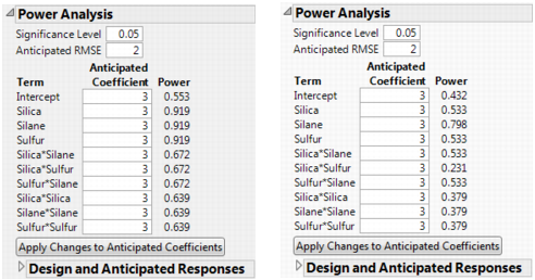
The power values for the actual design are uniformly smaller than for the intended design. For Silica and Sulfur, the power of the tests in the actual design is almost half the power in the intended design. For the Silica*Sulfur interaction, the power of the test in the actual design is 0.231, compared to 0.672 in the intended design. The actual design results in substantial loss of power in comparison with the intended design.
|
2.
|
In the window for the actual design, place your cursor on the scale for the vertical axis. When your cursor becomes a hand, right click. Select Edit > Copy Axis Settings.
|
|
3.
|
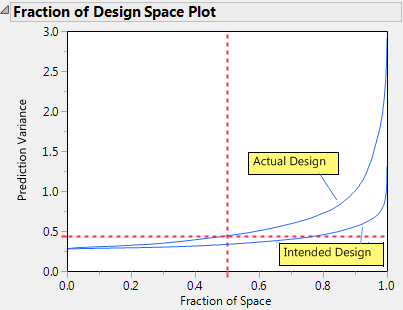
The plots are shown in Fraction of Design Space Plots, with the plot for the intended design at the top and for the actual design at the bottom.
|
4.
|
In both windows, select Maximize Desirability from the Prediction Variance Profile red triangle menu.
|
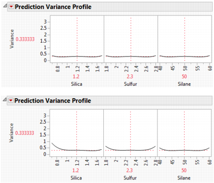
Prediction Variance Profile Maximized, Intended Design (Top) and Actual Design (Bottom) shows the maximum relative prediction variance for the intended and actual designs.
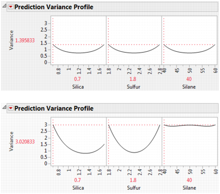
For both designs, the profilers identify the same point as one of the design points where the maximum prediction variance occurs: Silica=0.7, Sulfur=1.8, and Silane=40. The maximum prediction variance is 1.396 for the intended design, and 3.021 for the actual design. Note that there are other points where the prediction variance is maximized. The larger maximum prediction variance for the actual design means that predictions in parts of the design space are less accurate than they would have been had the intended design been conducted.
|
2.
|
In the window for the intended design, right-click in the plot and select Edit > Copy Frame Contents.
|
|
4.
|
Right-click in the plot and select Edit > Paste Frame Contents
|
Fraction of Design Space Plots shows the plot with annotations. Each Fraction of Design Space Plot shows the proportion of the design space for which the relative prediction variance falls below a specific value.
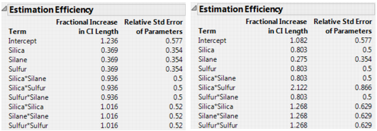
The Fractional Increase in CI Length compares the length of a parameter’s confidence interval as given by the current design to the length of such an interval given by an ideal design of the same run size. The length of the confidence interval, and consequently the Fractional Increase in CI Length, is affected by the number of runs. See Fractional Increase in CI Length. Despite the reduction in run size, for the actual design, the terms Silane, Silica*Silane, and Sulfur*Silane have a smaller increase than for the intended design. This is because the two runs that were removed to define the actual design had Silane set to its center point. By removing these runs, the widths of the confidence intervals for these parameters more closely resemble those of an ideal orthogonal design, which has no center points.
|
1.
|
Open the Color Map On Correlations outline.
|
|
3.
|
Click Remove Term.
|
The two color maps, shown in Color Map on Correlations, Intended Design (Left) and Actual Design (Right), are updated to show only the effects in the Model outline. Each plot shows the absolute correlations between effects colored using a blue to red intensity scale. Ideally, you would like zero or very small correlations between effects.
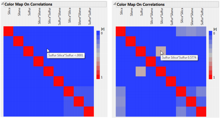
The absolute values of the correlations range from 0 (blue) to 1 (red). Hover over a cell to see the value of the absolute correlation. The color map for the actual design shows more absolute correlations that are large than does the color map for the intended design. For example, the correlation between Sulfur and Silica*Sulfur is < .0001 for the intended design, and 0.5774 for the actual design.
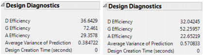
Note that both the number of runs and the model matrix factor into the calculation of efficiency measures. In particular, the D-, G-, and A- efficiencies are calculated relative to the ideal design for the run size of the given design. It is not necessarily true that larger designs are more efficient than smaller designs. However, for a given number of factors, larger designs tend to have smaller Average Variance of Prediction values than do smaller designs. For details on how efficiency measures are defined, see Design Diagnostics.
For this example, you have constructed a definitive screening design to determine which of six factors have an effect on the yield of an extraction process. The data are given in the Extraction Data.jmp sample data table, located in the Design Experiment folder. Because the design is a definitive screening design, each factor has three levels. See the Definitive Screening Designs section.
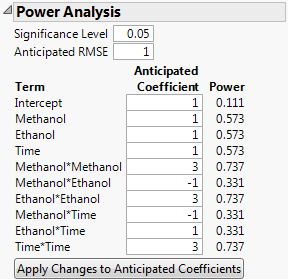
Although the experiment studies six factors, effect sparsity suggests that only a small subset of factors is active. Consequently, you feel comfortable investigating power in a model based on a smaller number of factors. Also, past studies on a related process provide strong evidence to suggest that three of the factors, Propanol, Butanol, and pH, have negligible main effects, do not interact with other factors, and do not have quadratic effects. This leads you to believe that the likely model contains main, interaction, and quadratic effects only for Methanol, Ethanol, and Time. You decide to investigate power in the context of a three-factor response surface model.
Use the Evaluate Design platform to determine the power of your design to detect strong quadratic effects for Methanol, Ethanol, or Time.
|
1.
|
|
2.
|
Select DOE > Evaluate Design.
|
|
3.
|
You can add Yield as Y, Response if you wish. But specifying the response has no effect on the properties of the design.
|
4.
|
Click OK.
|
|
5.
|
|
7.
|
|
8.
|
Click Apply Changes to Anticipated Coefficients.
|