Example of Partial Least Squares

This example is from spectrometric calibration, which is an area where partial least squares is very effective. Suppose you are researching pollution in the Baltic Sea. You would like to use the spectra of samples of sea water to determine the amounts of three compounds that are present in these samples.

The three compounds of interest are:

•	lignin sulfonate (ls), which is pulp industry pollution

•	humic acid (ha), which is a natural forest product

•	an optical whitener from detergent (dt)

The amounts of these compounds in each of the samples are the responses. The predictors are spectral emission intensities measured at a range of wavelengths (v1–v27).

For the purposes of calibrating the model, samples with known compositions are used. The calibration data consist of 16 samples of known concentrations of lignin sulfonate, humic acid, and detergent. Emission intensities are recorded at 27 equidistant wavelengths. Use the Partial Least Squares platform to build a model for predicting the amount of the compounds from the spectral emission intensities.

1.	Select Help > Sample Data Library and open Baltic.jmp.

Note: The data in the Baltic.jmp data table are reported in Umetrics (1995). The original source is Lindberg, Persson, and Wold (1983).

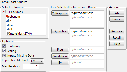
2.	Select Analyze > Multivariate Methods > Partial Least Squares.

3.	Assign ls, ha, and dt to the Y, Response role.

4.	Assign Intensities, which contains the 27 intensity variables v1 through v27, to the X, Factor role.

Click OK.

The Partial Least Squares Model Launch control panel appears.

6.	Select Leave-One-Out as the Validation Method.

Click Go.

A portion of the report appears in Partial Least Squares Report. Since the van der Voet test is a randomization test, your Prob > van der Voet T2 values can differ slightly from those in Partial Least Squares Report.

Partial Least Squares Report

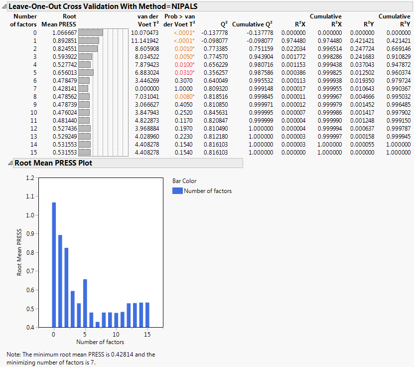
The Root Mean PRESS (predicted residual sum of squares) Plot shows that Root Mean PRESS is minimized when the number of factors is 7. This is stated in the note beneath the Root Mean PRESS Plot. A report called NIPALS Fit with 7 Factors is produced. A portion of that report is shown in Seven Extracted Factors.

The van der Voet T2 statistic tests to determine whether a model with a different number of factors differs significantly from the model with the minimum PRESS value. A common practice is to extract the smallest number of factors for which the van der Voet significance level exceeds 0.10 (SAS Institute Inc, 2011 and Tobias, 1995). If you were to apply this thinking here, you would fit a new model by entering 6 as the Number of Factors in the Model Launch panel.

Seven Extracted Factors

8.	Select Diagnostics Plots from the NIPALS Fit with 7 Factors red triangle menu.

This gives a report showing actual by predicted plots and three reports showing various residual plots. The Actual by Predicted Plot in Diagnostics Plots shows the degree to which predicted compound amounts agree with actual amounts.

Diagnostics Plots

9.	Select VIP vs Coefficients Plot from the NIPALS Fit with 7 Factors red triangle menu.

VIP vs Coefficients Plot

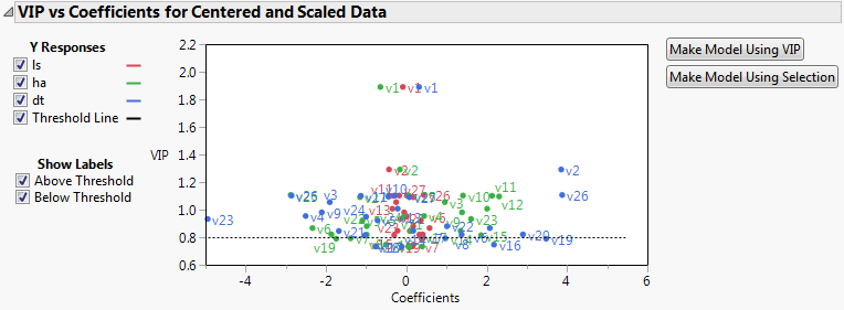
The VIP vs Coefficients plot helps identify variables that are influential relative to the fit for the various responses. For example, v23, v2, and v26 have both VIP values that exceed 0.8 and relatively large coefficients.

Launch the Partial Least Squares Platform

There are two ways to launch the Partial Least Squares platform:

•	Select Analyze > Multivariate Methods > Partial Least Squares.

•	Select Analyze > Fit Model and select Partial Least Squares from the Personality menu. This approach enables you to do the following:

‒	Enter categorical variables as Ys or Xs. Conduct PLS-DA by entering categorical Ys.

‒	Add interaction and polynomial terms to your model.

‒	Use the Standardize X option to construct higher-order terms using centered and scaled columns.

‒	Save your model specification script.

Some features on the Fit Model launch window are not applicable for the Partial Least Squares personality:

•	Weight, Nest, Attributes, Transform, and No Intercept.

Tip: You can transform a variable by right-clicking it in the Select Columns box and selecting a Transform option.

•	The following Macros: Mixture Response Surface, Scheffé Cubic, and Radial.

JMP Pro Partial Least Squares Launch Window (Imputation Method EM Selected)

The Partial Least Squares launch window contains the following options:

Y, Response

Enter numeric response columns. If you enter multiple columns, they are modeled jointly.

In JMP Pro, you can enter nominal response columns in the Fit Model launch window to conduct PLS-DA. For details, see PLS Discriminant Analysis (PLS-DA).

X, Factor

Enter the predictor columns. The Partial Least Squares launch window only allows numeric predictors.

In JMP Pro, you can enter nominal and ordinal model effects in the Fit Model launch window. Ordinal effects are treated as nominal.

Freq

If your data are summarized, enter the column whose values contain counts for each row.

Validation

Enter an optional validation column. A validation column must contain only consecutive integer values. Note the following:

‒	If the validation column has two levels, the smaller value defines the training set and the larger value defines the validation set.

‒	If the validation column has three levels, the values define the training, validation, and test sets in order of increasing size.

‒	If the validation column has more than three levels, then KFold Cross Validation is used. For information about other validation options, see Validation Method.

Note: If you click the Validation button with no columns selected in the Select Columns list, you can add a validation column to your data table. For more information about the Make Validation Column utility, see Basic Analysis.

Enter a column that creates separate reports for each level of the variable.

Centering

Centers all Y variables and model effects by subtracting the mean from each column. See Centering and Scaling.

Scaling

Scales all Y variables and model effects by dividing each column by its standard deviation. See Centering and Scaling.

Standardize X

(Fit Model launch window only) Select this option to center and scale all columns that are used in the construction of model effects. If this option is not selected, higher-order effects are constructed using the original data table columns. Then each higher-order effect is centered or scaled, based on the selected Centering and Scaling options. Note that Standardize X does not center or scale Y variables. See Standardize X.

Impute Missing Data

Replaces missing data values in Ys or Xs with nonmissing values. Select the appropriate method from the Imputation Method list.

If Impute Missing Data is not selected, rows that are missing observations on any X variable are excluded from the analysis and no predictions are computed for these rows. Rows with no missing observations on X variables but with missing observations on Y variables are also excluded from the analysis, but predictions are computed.

Imputation Method

(Appears only when Impute Missing Data is selected) Select from the following imputation methods:

‒	Mean: For each model effect or response column, replaces the missing value with the mean of the nonmissing values.

‒

EM: Uses an iterative Expectation-Maximization (EM) approach to impute missing values. On the first iteration, the specified model is fit to the data with missing values for an effect or response replaced by their means. Predicted values from the model for Y and the model for X are used to impute the missing values. For subsequent iterations, the missing values are replaced by their predicted values, given the conditional distribution using the current estimates.

For the purpose of imputation, polynomial terms are treated as separate predictors. When a polynomial term is specified, that term is calculated from the original data, or, if Standardize X is checked, from the standardized column values. If a row has a missing value for a column involved in the definition of the polynomial term, then that entry is missing for the polynomial term. Imputation is conducted using polynomial terms defined in this way.

For more details about the EM approach, see Nelson, Taylor, and MacGregor (1996).

Max Iterations

(Appears only when EM is selected as the Imputation Method) Enables you to set the maximum number of iterations used by the algorithm. The algorithm terminates if the maximum difference between the current and previous estimates of missing values is bounded by 10^-8.

After completing the launch window and clicking OK, the Model Launch control panel appears. See Model Launch Control Panel.

Centering and Scaling

The Centering and Scaling options are selected by default. This means that predictors and responses are centered and scaled to have mean 0 and standard deviation 1. Centering the predictors and the responses places them on an equal footing relative to their variation. Without centering, both the variable’s mean and its variation around that mean are involved in constructing successive factors. To illustrate, suppose that Time and Temp are two of the predictors. Scaling them indicates that a change of one standard deviation in Time is approximately equivalent to a change of one standard deviation in Temp.

Standardize X

When the Partial Least Square personality is selected in the Fit Model window, the Standardize X option is selected by default. This ensures that all columns entered as model effects and that all columns that are involved in an interaction or polynomial term are standardized.

Suppose that you have two columns, X1 and X2, and you enter the interaction term X1*X2 as a model effect in the Fit Model window. When the Standardize X option is selected, both X1 and X2 are centered and scaled before forming the interaction term. The interaction term that is formed is calculated as follows:

All model effects are then centered or scaled, in accordance with your selections of the Centering and Scaling options, prior to inclusion in the model.

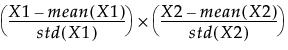
If the Standardize X option is not selected, and Centering and Scaling are both selected, then the term that is entered into the model is calculated as follows: