Sometimes measurements on the experimental units that are intended for an experiment are available. These measurements might affect the experimental response. It is useful to include these variables, called covariates, as design factors. Although you cannot directly control these values, you can ensure that the levels of the other design factors are chosen to yield the most precise estimates of all the effects.
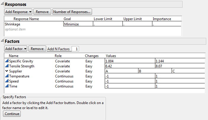
In this example, you are interested in modeling the Shrinkage of parts produced by an injection molding process. The Thermoplastic.jmp sample data table in the Design Experiment folder lists 25 batches of raw (thermoplastic) material for potential use in your study. For each batch, material was removed to obtain measurements of Specific Gravity and Tensile Strength. A third covariate, Supplier, is also available.
You want to study the effects of three controllable factors, Temperature (mold temperature), Speed (screw speed), and Time (hold time), on Shrinkage. But you also want to study the effects of the covariates: Specific Gravity, Tensile Strength, and Supplier. Your resources allow for 12 runs.
|
1.
|
|
2.
|
Select DOE > Custom Design.
|
|
3.
|
|
4.
|
|
5.
|
|
6.
|
|
7.
|
Type 3 next to Add N Factors.
|
|
8.
|
Click Add Factor > Continuous.
|
|
9.
|
|
10.
|
Click Continue.
|
|
11.
|
Type 12 next to Number of Runs.
|
Note: Setting the Random Seed in step 12 and Number of Starts in step 13 reproduces the exact results shown in this example. In constructing a design on your own, these steps are not necessary.
|
12.
|
(Optional) From the Custom Design red triangle menu, select Set Random Seed, type 84951, and click OK.
|
|
13.
|
(Optional) From the Custom Design red triangle menu, select Number of Starts, type 40, and click OK.
|
|
14.
|
Click Make Design.
|

|
15.
|
Open the Design Evaluation > Color Map On Correlations outline.
|

The seven terms corresponding to main effects appear in the upper left corner of the color map. Notice that these seven terms are close to orthogonal. The largest absolute correlation is between Tensile Strength and Supplier 2. This absolute correlation of about 0.43 is a consequence of the available covariate values.
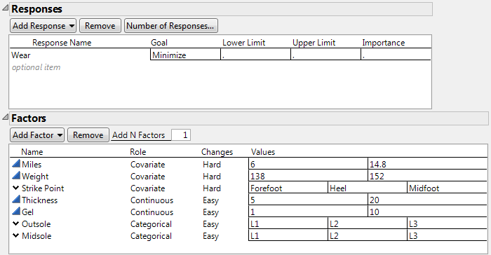
In this example, you construct a design for developing a running shoe for serious runners that has good wear (Wear) properties. Your experimental factors include the following:
|
•
|
sole thickness (Thickness)
|
|
•
|
outsole material (Outsole)
|
|
•
|
midsole material (Midsole)
|
Your company has collected data on 100 suitable runners willing to participate in your study. The concomitant variables (covariates) measured on these runners are average daily miles run (Miles), weight (Weight), and the foot’s strike point (Strike Point).
|
1.
|
|
2.
|
Select DOE > Custom Design.
|
|
3.
|
|
4.
|
|
5.
|
|
6.
|
|
7.
|
For one of the factors Miles, Weight, and Strike Point, under Changes, click Easy and change it to Hard.
|
|
8.
|
To add the remaining factors manually, follow step 9 through step 17. Or, to load factors from a saved table, select Load Factors from the red triangle menu next to Custom Design. Open the Runners Factors.jmp sample data table, located in the Design Experiment folder. If you select Load Factors, skip step 9 through step 17.
|
|
9.
|
Type 2 next to Add N Factors.
|
|
10.
|
Click Add Factor > Continuous.
|
|
11.
|
|
12.
|
|
13.
|
|
14.
|
Type 2 next to Add N Factors.
|
|
15.
|
Click Add Factor > Categorical > 3 Level.
|
|
16.
|
Keep the default Values for these factors.
|
17.
|
Click Continue.
|
|
18.
|
Select Interactions > 2nd.
|
Note: Setting the Random Seed in step 21 and Number of Starts in step 22 reproduces the exact results shown in this example. In constructing a design on your own, these steps are not necessary.
|
21.
|
(Optional) From the Custom Design red triangle menu, select Set Random Seed, type 12345, and click OK.
|
|
22.
|
(Optional) From the Custom Design red triangle menu, select Number of Starts and set it to 1(if it is not already set to that number). Click OK.
|
|
23.
|
Click Make Design.
|

Of the 100 runners, 32 are selected based on their covariate values. The rows corresponding to the selected runners are selected in the RunnersCovariates.jmp sample data table. Settings of the experimental factors Thickness, Gel, Insole, and Outsole are determined so that the design is optimal for the model described in the Model Outline.
|
24.
|
With the RunnersCovariates.jmp sample data table as the active table, select Analyze > Distribution.
|
|
25.
|
Select all three columns as Y, Columns.
|
|
26.
|
Check Histograms Only.
|
|
27.
|
Click OK.
|
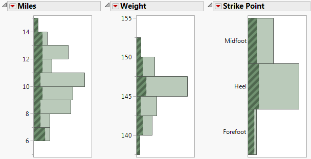
The histograms indicate that all of the runners with Miles of 14.0 or higher were selected. Runners at the extremes of the Weight distribution were selected. Almost all of the runners with a Strike Point of Forefoot were selected. Notice that the design is somewhat balanced in terms of Strike Point.
|
1.
|
Select File > New > Data Table.
|
|
2.
|
|
3.
|
Change the column name to Run Order.
|
|
4.
|
|
5.
|
Type 16 next to To.
|
|
6.
|
Click OK.
|
|
7.
|
Select DOE > Custom Design.
|
|
8.
|
Click Add Factor > Covariate.
|
|
9.
|
|
10.
|
Type 7 next to Add N Factors.
|
|
11.
|
Click Add Factor > Continuous.
|
|
12.
|
Click Continue.
|
|
13.
|
Open the Alias Terms outline.
|
|
14.
|
Select all of the effects in the list and click Remove Term.
|
Note: Setting the Random Seed in step 15 and Number of Starts in step 16 reproduces the exact results shown in this example. In constructing a design on your own, these steps are not necessary.
|
15.
|
(Optional) From the Custom Design red triangle menu, select Set Random Seed, type 1084680980, and click OK.
|
|
16.
|
(Optional) From the Custom Design red triangle menu, select Number of Starts, type 30000, and click OK.
|
|
17.
|
Click Make Design.
|

|
18.
|
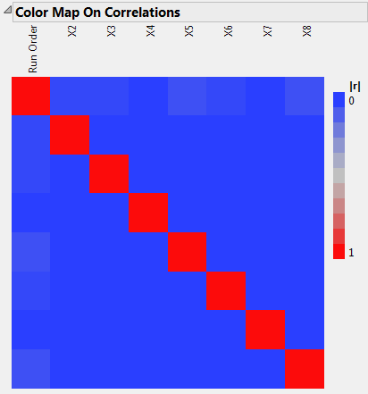
Open the Design Evaluation > Color Map On Correlations outline.
|
|
‒
|
|
‒
|
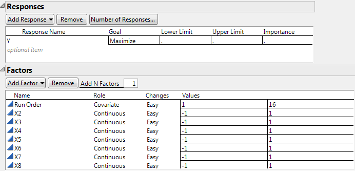
Run Order, the linear time trend variable, has extremely low absolute correlation with X2 through X8.
|
|
19.
|
Open the Design Evaluation > Estimation Efficiency outline.
|
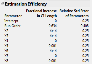
The small absolute correlations of Run Order with X2 through X8 result in very small increases in confidence interval lengths, relative to an ideal orthogonal design. The increases in the lengths of confidence intervals for X2 through X8 are all less than 0.1%.