Whether you remove or retain outliers, you must locate them. There are many ways to visually inspect for outliers. For example, box plots, histograms, and scatter plots can sometimes easily display these extreme values. See the Visualizing Your Data chapter of the Discovering JMP book for more information.
The Probe.jmp sample data table contains 387 characteristics (the Responses column group) measured on 5800 semiconductor wafers. The Lot ID and Wafer Number columns uniquely identify the wafer. You are interested in identifying outliers within a select group of columns of the data set. Use the Explore Outliers utility to identify outliers that can then be examined using the Distribution platform.
|
1.
|
|
2.
|
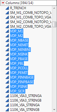
Expand the Responses column group and select columns VDP_M1 through VDP_SICR. You should have 14 columns selected (see Selected Columns).
|
|
3.
|
Select Cols > Modeling Utilities > Explore Outliers.
|
|
4.
|
Click Quantile Range Outliers.
|
|
5.
|
Select Show only columns with outliers to limit the list of columns to only those that contain outliers.
|
|
7.
|
Click Add Highest Nines to Missing Value Codes.
|
A JMP Alert indicates that you should use the Save As command to preserve your original data.
|
8.
|
Click OK.
|
|
9.
|
|
10.
|
Select Restrict search to integers.
|
|
11.
|
Deselect Restrict search to integers.
|
|
2.
|
Click Select Rows.
|
|
3.
|
Select Analyze > Distribution.
|
|
4.
|
Assign the selected columns to the Y, Columns role. Because you selected these column names in the Quantile Range Outliers report, they are already selected in the Distribution launch window.
|
|
5.
|
Click OK.
|
Distribution of Columns with Outliers Selected shows a simplified version of the report.
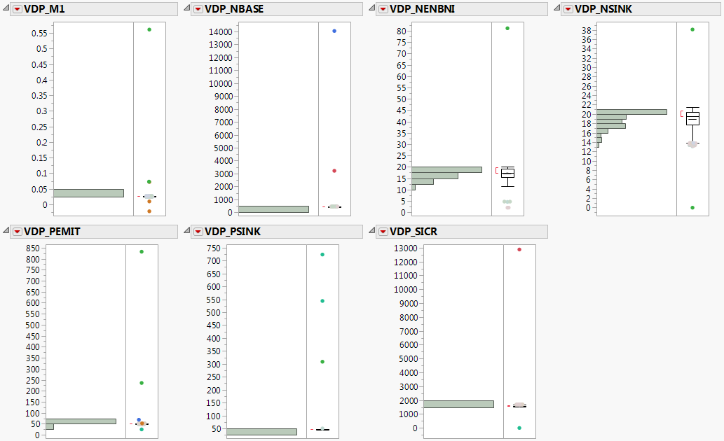
In columns VDP_M1 and VDP_PEMIT, notice that the selected outliers are somewhat close to the majority of data. For the rest of the columns, the selected outliers appear distant enough to exclude them from your analyses.
|
1.
|
|
2.
|
With the remaining columns selected in the report, click Exclude Rows.
|
|
4.
|
Click Rescan.
|
|
5.
|
|
2.
|
In the Quantile Range Outliers report, click Exclude Rows.
|
|
4.
|
Select Script > Redo Analysis.
|
Distributions of Columns with Outliers Excluded shows a simplified version of the report.

Launch the Explore Outliers utility by first selecting the columns of interest, and then selecting Cols > Modeling Utilities > Explore Outliers.
The Quantile Range Outliers method of outlier detection uses the quantile distribution of the values in a column to locate the extreme values. Quantiles are useful for detecting outliers because there is no distributional assumption associated with them. Data are simply sorted from smallest to largest. For example, the 20th quantile is the value at which 20% of values are smaller. Extreme values are found using a multiplier of the interquantile range, the distance between two specified quantiles. For more details about how quantiles are computed, see Statistical Details for Quantiles in Distributions.
The Quantile Range Outliers panel enables you to specify how outliers are to be calculated and how you want to manage them. Quantile Range Outliers Window shows the default Quantile Range Outliers window.

An outlier is considered any value more than Q times the interquantile range from the lower and upper quantiles. You can adjust the value of Q and the size of the interquantile range.
The multiplier that helps determine values as outliers. Outliers are considered Q times the interquantile range past the Tail Quantile and  values. Large values of Q provide a more conservative set of outliers than small values. The default is 3.
Turns on the exclude row state for the selected rows. Click Rescan to update the Quantile Range Outliers report.
Adds the selected outliers to the missing value codes column property. Use this option to identify known missing value or error codes within the data. Missing value and error codes are often integers and are sometimes either a positive or negative series of nines. Click Rescan to update the Quantile Range Outliers report.
Changes the outlier value to a missing value in the data table. Use caution when changing values to missing. Change values to missing only if the data are known to be invalid or inaccurate. Click Rescan to update the Quantile Range Outliers report.
Adds the selected outlier values to the missing value codes column property. You must click Rescan to update the Quantile Range Outliers report.
Note: The first time you use choose an action (such as Change to Missing or Exclude Rows) to change your data, the alert window warns you to use the Save As command to save your data table as a new file to preserve a copy of your original data. When this window appears, click OK. If you decide to save your new data file, select File > Save As and save the file with a new name.
Robust estimates of parameters are less sensitive to outliers than non-robust estimates. Robust Fit Outliers provides several types of robust estimates of the center and spread of your data to determine those values that can be considered extreme. Robust Fit Outliers Window shows the default Robust Fit Outliers window.
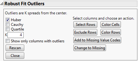
Given a robust estimate of the center and spread, outliers are defined as those values that are K times the robust spread from the robust center. The Robust Fit Outliers window provides several options for calculating the robust estimates and multiplier K as well as provides tools to manage the outliers found.
The multiplier that determines outliers as K times the spread away from the center. Large values of K provide a more conservative set of outliers than small values. The default is 4.
Sets the Exclude Row state for outliers in the selected columns in the data table. Click Rescan to update the Robust Estimates and Outliers report.
Adds the selected outliers to the missing value codes column property for the selected columns. Use this option to identify known missing value or error codes within the data. Click Rescan to update the Robust Estimates and Outliers report.
Changes the outlier value to a missing value in the data table. Click Rescan to update the Robust Estimates and Outliers report.
You can save the distances to the data table by selecting the Save option from the Mahalanobis Distances red triangle menu.
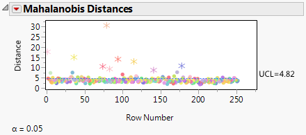
Multivariate Robust Outliers Mahalanobis Distance Plot shows the Mahalanobis distances of 16 different columns. The plot contains an upper control limit (UCL) of 4.82.This UCL is meant to be a helpful guide to show where potential outliers might be. However, you should use your own discretion to determine which values are outliers. For more details about this upper control limit (UCL), see Mason and Young (2002).
The basic approach of outlier detection is to consider points distant from other points as outliers. One way of determining the distance of a point to most points is identifying the distance to its k-nearest neighbors. The Multivariate k-Nearest Neighbor Outliers utility displays the Euclidean distances between each point and that point’s nearest K neighbors, where  , skipping values by the Fibonacci sequence to avoid too many plots.
This approach is sensitive to the value of k. If k is too small, then a small number of nearby outliers can decrease the distance displayed and hide the outliers. If k is too large, then it is possible for points that appear to be outliers to actually be within natural clusters with smaller than k data points. In other words, small k can under-identify outliers; large k can over-identify outliers. Higher values of k, however, can reduce the impact of insignificant variables included in the analysis.
To launch the utility, select Multivariate k-Nearest Neighbor Outliers from the Commands section of the Explore Outliers window. Specify the value of k (the default is 8) and click OK.
The K Nearest Neighbors report shows the distance between each point and that point’s nearest neighbor, the second nearest neighbor, up to the kth nearest neighbor. The data points that consistently have a large distance from their neighbors are likely to be outliers.
You can select the suspected outliers using your mouse in the plot. Explore these selected data points further by clicking Scatterplot Matrix.
If you determine the selected data points are outliers, you can exclude them from further analysis by clicking Exclude Selected Rows.
After the rows are excluded, you are given the option to either rerun the analysis or close the utility. Rerunning the analysis recalculates the k-nearest neighbors for all points except those excluded rows. Note that unless you hide the excluded rows in the data table, they still appear in the graph.
The Water Treatment.jmp data set contains daily measurement values of 38 sensors in an urban waste water treatment plant. You are interested in exploring these data for potential outliers. Potential outliers could include sensor failures, storms, and other situations.
|
1.
|
|
2.
|
Select the columns in the Sensor Measurements column group.
|
|
3.
|
Select Cols > Modeling Utilities > Explore Outliers > Multivariate k-Nearest Neighbor Outliers.
|
|
5.
|
Click OK.
|

Notice the three extreme outliers selected in the k-Nearest Neighbors plots in Outliers in Multivariate k-Nearest Neighbor Outliers Example. Each of these three data points corresponds to a date where the secondary settler in the water treatment plant was reported as malfunctioning. Because these three data points are due to faulty equipment, exclude them from future analyses.
|
6.
|
Select the three extreme outliers and click Exclude Selected Rows.
|
|
7.
|
Click Rerun.
|
|
9.
|
Click OK.
|
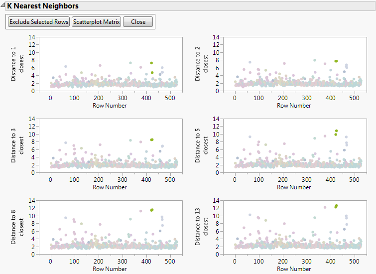
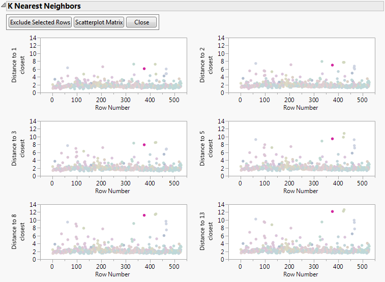
Now locate the two light-green outliers close to row 400. Notice how they tend to stay close to each other as k increases. Even though these data points have a relatively high Distance to 13 closest, these two points have been identified as solids overloads to the water treatment plant. Since these two points are due to real situations, do not exclude them. However, you might want to keep them in mind during future analyses.
|
11.
|
Click Scatterplot Matrix.
|
|
12.
|
Scroll down to the bottom of the matrix. Notice how extremely low the RD-SED-G value is for this point. Not only does this point have an extremely low RD-SED-G value, it is also one of the few data points that have such low value.
|
|
13.
|
Scroll to the right to look at the relationship between RD-SED-G and SED-S. You can see that this point has a low RD-SED-G and high SED-S value. There does appear to be a relationship between these two variables. It is uncommon to have a low RD-SED-G or a high SED-S value, but it is not impossible. There is not enough evidence to exclude this point from your analyses.
|