This option fits a Crow-AMSAA model (MIL-HDBK-189, 1981). A Crow-AMSAA model is a nonhomogeneous Poisson process with failure intensity as a function of time t given by ρ(t) = λβtβ-1. Here, λ is a scale parameter and β is a growth parameter. This function is also called a Weibull intensity, and the process itself is also called a power law process (Rigdon and Basu, 2000; Meeker and Escobar, 1998). Note that the Recurrence platform fits the Power Nonhomogeneous Poisson Process, which is equivalent to the Crow-AMSAA model, though it uses a different parameterization. See Fit Model in Recurrence Analysis for details.
The intensity function is a concept applied to repairable systems. Its value at time t is the limiting value of the probability of a failure in a small interval around t, divided by the length of this interval; the limit is taken as the interval length goes to zero. You can think of the intensity function as measuring the likelihood of the system failing at a given time. If β < 1, the system is improving over time. If β > 1, the system is deteriorating over time. If β = 1, the rate of occurrence of failures is constant.
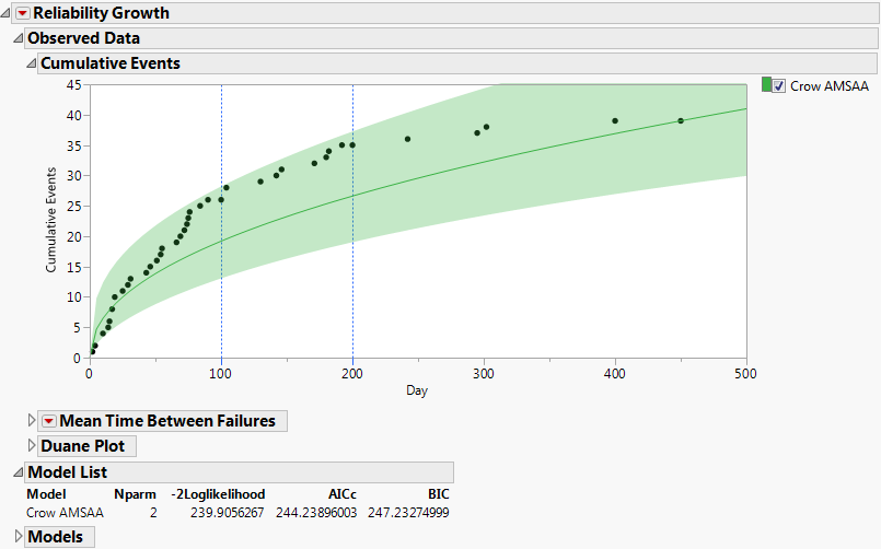
When the Crow AMSAA option is selected, the Cumulative Events plot updates to show the cumulative events curve estimated by the model. For each time point, the shaded band around this curve defines a 95% confidence interval for the true cumulative number of events at that time. The Model List report also updates. Crow AMSAA Cumulative Events Plot and Model List Report shows the Observed Data report for the data in TurbineEngineDesign1.jmp.
A Crow-AMSAA report opens within the Models report. If Time to Event Format is used, the Crow AMSAA report shows an MTBF plot with both axes scaled logarithmically. See Show MTBF Plot.
This plot is displayed by default (MTBF Plot). For each time point, the shaded band around the MTBF plot defines a 95% confidence interval for the true MTBF at time t. If Time to Event Format is used, the plot is shown with both axes logarithmically scaled. With this scaling, the MTBF plot is linear. If Dates Format is used, the plot is not logarithmically scaled.
To see why the MTBF plot is linear when logarithmic scaling is used, consider the following. The mean time between failures is the reciprocal of the intensity function. For the Weibull intensity function, the MTBF is 1/(λβtβ-1), where t represents the time since testing initiation. It follows that the logarithm of the MTBF is a linear function of log(t), with slope 1 ‑ β. The estimated MTBF is defined by replacing the parameters λ and β by their estimates. So the log of the estimated MTBF is a linear function of log(t).
Maximum likelihood estimates for lambda (λ), beta (β), and the Reliability Growth Slope (1 ‑ β), appear in the Estimates report below the plot. (See MTBF Plot.) Standard errors and 95% confidence intervals for λ, β, and 1 ‑ β are given. For details about calculations, see Parameter Estimates for Crow-AMSAA Models.
This plot shows the estimated intensity function (Intensity Plot). The Weibull intensity function is given by ρ(t) = λβtβ-1, so it follows that log(Intensity) is a linear function of log(t). If Time to Event Format is used, both axes are scaled logarithmically.
This plot shows the estimated cumulative number of events (Cumulative Events Plot). The observed cumulative numbers of events are also displayed on this plot. If Time to Event Format is used, both axes are scaled logarithmically.
For the Crow-AMSAA model, the cumulative number of events at time t is given by λtβ. It follows that the logarithm of the cumulative number of events is a linear function of log(t). So, the plot of the estimated Cumulative Events is linear when plotted against logarithmically scaled axes.
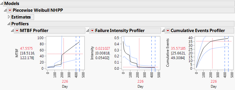
Three profilers are displayed, showing estimated MTBF, Failure Intensity, and Cumulative Events (Profilers). These profilers do not use logarithmic scaling. By dragging the red vertical dashed line in any profiler, you can explore model estimates at various time points; the value of the selected time point is shown in red beneath the plot. Also, you can set the time axis to a specific value by pressing the CTRL key while you click in the plot. A blue vertical dashed line denotes the time point of the last observed failure.
The profilers also display 95% confidence bands for the estimated quantities. For the specified time setting, the estimated quantity (in red) and 95% confidence limits (in black) are shown to the left of the profiler. For further details, see Profilers.
Note that you can link these profilers by selecting Factor Settings > Link Profilers from any of the profiler red triangle menus. For further details about the use and interpretation of profilers, see Factor Profiling in the Standard Least Squares chapter of the Fitting Linear Models book. Also see the Profilers book.
A confidence interval for the MTBF at the point when testing concludes is often of interest. For uncensored failure time data, this report gives an estimate of the Achieved MTBF and a 95% confidence interval for the Achieved MTBF. You can specify a 100*(1-α)% confidence interval by entering a value for Alpha. The report is shown in Achieved MTBF Report. For censored data, only the estimated MTBF at test termination is reported.
There are infinitely many possible failure-time sequences from an NHPP; the observed data represent only one of these. Suppose that the test is failure terminated at the nth failure. The confidence interval computed in the Achieved MTBF report takes into account the fact that the n failure times are random. If the test is time terminated, then the number of failures as well as their failure times are random. Because of this, the confidence interval for the Achieved MTBF differs from the confidence interval provided by the MTBF Profiler at the last observed failure time. Details can be found in Crow (1982) and Lee and Lee (1978).
The Goodness of Fit report tests the null hypothesis that the data follow an NHPP with Weibull intensity. Depending on whether one or two time columns are entered, either a Cramér-von Mises (see Cramér-von Mises Test for Data with Uncensored Failure Times) or a chi-squared test (see Chi-Squared Goodness of Fit Test for Interval-Censored Failure Times) is performed.
The entry below the p-Value heading indicates how unlikely it is for the test statistic to be as large as what is observed if the data come from a Weibull NHPP model. The platform computes p-values up to 0.25. If the test statistic is smaller than the value that corresponds to a p-value of 0.25, the report indicates that its p-value is >=0.25. Details about this test can be found in Crow (1975).
Goodness of Fit Report - Cramér-von Mises Test shows the goodness-of-fit test for the fit of a Crow-AMSAA model to the data in TurbineEngineDesign1.jmp. The computed test statistic corresponds to a p-value that is less than 0.01. We conclude that the Crow-AMSAA model does not provide an adequate fit to the data.
In the Crow-AMSAA model, the maximum likelihood estimate (MLE) of β is biased. This option fits a Crow AMSAA model where β is adjusted for bias.
Crow AMSAA with Modified MLE Report shows a Crow-AMSAA with Modified MLE fit to the data in TurbineEngineDesign1.jmp.
The formula for the bias-corrected estimate of β depends on whether the test is failure terminated or time terminated. See Parameter Estimates for Crow-AMSAA with Modified MLE for details.
When the Crow-AMSAA with Modified MLE option is selected, the Cumulative Events Plot updates to display this model. The Model List also updates. The Crow-AMSAA with Modified MLE report opens to show the MTBF plot for the Crow-AMSAA with Modified MLE fit; this plot is described in the section Show MTBF Plot.
In addition to Show MTBF plot, available options are Show Intensity Plot, Show Cumulative Events Plot, Show Profilers, Achieved MTBF, and Goodness of Fit. These reports are described under Crow AMSAA. Details of how the modified MLEs are used to construct these reports are given in Parameter Estimates for Crow-AMSAA with Modified MLE. Details about the Goodness of Fit and Achieved MTBF reports specific to the modified MLE option are given below.
Because the Crow-AMSAA with Modified MLE option is only available when the data are entered as a single Time to Event or Timestamp column, the Goodness of Fit test is a Cramér-von Mises test. Because the estimate of β is used in this test is bias-corrected, the test results are identical to those of the Goodness of Fit test for the Crow-AMSAA model.
When the Fixed Parameter Crow-AMSAA option is selected, the Cumulative Events Plot updates to display this model. The Model List also updates. The Fixed Parameter Crow-AMSAA report opens to show the MTBF plot for the Crow-AMSAA fit; this plot is described in the section Show MTBF Plot.
In addition to Show MTBF plot, available options are Show Intensity Plot, Show Cumulative Events Plot, and Show Profilers. The construction and interpretation of these plots is described under Crow AMSAA.
The initial parameter estimates are the MLEs from the Crow-ASMAA fit. Either parameter can be fixed by checking the box next to the desired parameter and then entering the desired value. The model is re-estimated and the MTBF plot updates to describe this model. Fixed Parameter Crow AMSAA Report shows a fixed-parameter Crow-AMSAA fit to the data in TurbineEngineDesign1.jmp, with the value of beta set at 0.4.
The Piecewise Weibull NHPP model can be fit when a Phase column specifying at least two values has been entered in the launch window. Crow-AMSAA models are fit to each of the phases under the constraint that the cumulative number of events at the start of a phase matches that number at the end of the preceding phase. For proper display of phase transition times, the first row for every Phase other than the first must give that phase’s start time. See Multiple Test Phases.
When the report is run, the Cumulative Events plot updates to show the piecewise model. Blue vertical dashed lines show the transition times for each of the phases. The Model List also updates. See Cumulative Events Plot and Model List Report, where both a Crow-AMSAA model and a piecewise Weibull NHPP model have been fit to the data in TurbineEngineDesign1.jmp. Note that both models are compared in the Model List report.
By default, the Piecewise Weibull NHPP report shows the estimated MTBF plot, with color coding to differentiate the phases. The Estimates report is shown below the plot. (See Piecewise Weibull NHPP Report.)
The MTBF plot and an Estimates report open by default when the Piecewise Weibull NHPP option is chosen (Piecewise Weibull NHPP Report). When Time to Event Format is used, the axes are logarithmically scaled. For further details about the plot, see Show MTBF Plot.
The Estimates report gives estimates of the model parameters. Note that only the estimate for the value of λ corresponding to the first phase is given. In the piecewise model, the cumulative events at the end of one phase must match the number at the beginning of the subsequent phase. Because of these constraints, the estimate of λ for the first phase and the estimates of the βs determine the remaining λs.
The method used to calculate the estimates, their standard errors, and the confidence limits is similar to that used for the simple Crow-AMSAA model. For further details, see Parameter Estimates for Crow-AMSAA Models. The likelihood function reflects the additional parameters and the constraints on the cumulative numbers of events.
The Intensity plot shows the estimated intensity function and confidence bounds over the design phases. The intensity function is generally discontinuous at a phase transition. Color coding facilitates differentiation of phases. If Time to Event Format is used, the axes are logarithmically scaled. For further details, see Show Intensity Plot.
The Cumulative Events plot shows the estimated cumulative number of events, along with confidence bounds, over the design phases. The model requires that the cumulative events at the end of one phase match the number at the beginning of the subsequent phase. Color coding facilitates differentiation of phases. If Time to Event Format is used, the axes are logarithmically scaled. For further details, see Show Cumulative Events Plot.
Three profilers are displayed, showing estimated MTBF, Failure Intensity, and Cumulative Events. These profilers do not use logarithmic scaling. For more detail on interpreting and using these profilers, see the section Show Profilers.
It is important to note that, due to the default resolution of the profiler plot, discontinuities are not displayed clearly in the MTBF or Failure Intensity Profilers. In the neighborhood of a phase transition, the profiler trace shows a nearly vertical, but slightly sloped, line; this line represents a discontinuity. (See Profilers.) Such a line at a phase transition should not be used for estimation. You can obtain a higher-resolution display making these lines appear more vertical as follows. Press CTRL while clicking in the profiler plot, and then enter a larger value for Number of Plotted Points in the dialog window. (See Factor Settings Window, where we have specified 500 as the Number of Plotted Points.)
|
•
|
Suppose that a single column is entered as Time to Event or Timestamp. Then the start time for a new phase, with a zero Event Count, must appear in the first row for that phase. See the sample data table ProductionEquipment.jmp, in the Reliability subfolder, for an example.
|
|
•
|
If two columns are entered, then an interval whose left endpoint is that start time must appear in the first row, with the appropriate event count. The sample data table TurbineEngineDesign2.jmp, found in the Reliability subfolder, provides an example. Also, see Piecewise NHPP Weibull Model Fitting with Interval-Censored Data.
|
By default, the Reinitialized Weibull NHPP report shows the estimated MTBF plot, with color coding to differentiate the phases. The Estimates report is shown below the plot. (See Reinitialized Weibull NHPP Report, which uses the ProductionEquipment.jmp sample data file from the Reliability subfolder.)
The MTBF plot opens by default when the Reinitialized Weibull NHPP option is chosen. For further details about the plot, see Show MTBF Plot.
The Estimates report gives estimates of λ and β for each of the phases. For a given phase, λ and β are estimated using only the data from that phase. The calculations assume that the phase begins at time 0 and reflect whether the phase is failure or time terminated, as defined by the data table structure (see Test Phases). Also shown are standard errors and 95% confidence limits. These values are computed as described in Parameter Estimates for Crow-AMSAA Models.
The Intensity plot shows the estimated intensity functions for the phases, along with confidence bands. Because the intensity functions are computed based only on the data within a phase, they are discontinuous at phase transitions. Color coding facilitates differentiation of phases. For further details, see Show Intensity Plot.
The Cumulative Events plot for the Reinitialized Weibull NHPP model portrays the estimated cumulative number of events, with confidence bounds, over the design phases in the following way. Let t represent the time since the first phase of testing began. The model for the phase in effect at time t is evaluated at time t. In particular, the model for the phase in effect is not evaluated at the time since the beginning of the specific phase; rather it is evaluated at the time since the beginning of the first phase of testing.
Three profilers are displayed, showing estimated MTBF, Failure Intensity, and Cumulative Events. Note that the Cumulative Events Profiler is constructed as described in the Cumulative Events Plot section. In particular, the cumulative number of events at the beginning of one phase is matched to the number at the end of the previous phase. For further details, see Show Profilers.
|
•
|
a Phase has not been entered in the launch window
|
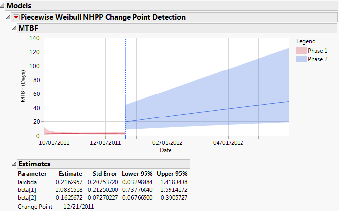
The default Piecewise Weibull NHPP Change Point Detection report shows the MTBF plot and Estimates. (See Piecewise Weibull NHPP Change Point Detection Report, which uses the data in BrakeReliability.jmp, found in the Reliability subfolder.) Note that the Change Point, shown at the bottom of the Estimates report, is estimated as 12/21/2011. The standard errors and confidence intervals consider the change point to be known. The plot and the Estimates report are described in the section Piecewise Weibull NHPP.