This section describes how to connect to a database and import the data. Refer to Build SQL Queries in Query Builder for details about interactively building queries.
Your operating system provides an interface for JMP to communicate with databases using ODBC data sources. Create and configure data sources with operating system software. For example, on Windows 7, use Control Panel > System and Security > Administrative Tools > Data Sources (ODBC); on the Macintosh, use Applications > Utilities > ODBC Manager.
|
1.
|
Select File > Database > Open Table. The Connections box lists data sources that you have connected to in the current JMP session.
|
|
2.
|
Click New Connection.
|
|
3.
|
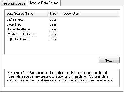
(Windows) In the Select Data Source window (Select a Data Source (Windows)), click the Machine Data Source tab, select the data source, click OK, enter the user name and password, and then click OK.
|
|
1.
|
Select File > Database > Open Table.
|
|
2.
|

Note: The Fetch Procedures check box is disabled if the ODBC driver does not support fetching procedures.
|
3.
|
If the desired data source is not listed in the Connections box, click Connect to choose a data source. The method of choosing a data source depends on your operating system. Select a data source and click OK.
|
|
5.
|
Control which tables are listed by choosing the options in the Include in Table List group of check boxes. Different drivers interpret these labels differently. Your options are as follows:
|
User Tables When clicked, displays all available user tables in the Tables list. User tables are specific to which user is logged on to the computer.
Views When clicked, displays “views” in the Tables list along with all other file types that can be opened. “Views” are virtual tables that are query result sets updated each time you open them. They are used to extract and combine information from one or more tables.
System Tables When clicked, displays all available system tables in the Tables list. System tables are tables that can be used by all users or by a system-wide service.
Synonyms When clicked, displays all available ORACLE synonyms in the Tables list.
Sampling Enter the percentage of rows that you want to appear in the list of tables. Selecting this option speeds up queries in large databases. JMP uses the sampling method supported by the database. The check box is unavailable when the database does not support sampling.
Note: If you are connected to a dBase database, select the database folder to which you would like to connect. Individual files are grayed out and cannot be selected.
|
7.
|
Click Open Table to import all the data in the selected table, or click Advanced to specify a subset of the table to be imported. Some databases require that you enter the user ID and password to access the data.
|
You might see a short delay when opening large tables. To see the status of all active ODBC queries, select View > Running Queries.
This section describes how to write SQL statements to retrieve data. To interactively query data without writing SQL statements, use Query Builder. You can also start creating a query in Query Builder and then add your own SQL. See Write SQL Statements in Query Builder for details.
|
1.
|
Select File > Database > Open Table.
|
|
2.
|
|
3.
|
From the Database Open Table window, click the Advanced button to open specific subsets of a table.
|
|
4.
|
Either type in a valid SQL statement, or modify the default statement. Import Data from a Database shows a default SQL Select statement appropriate for the selected file. See Structured Query Language (SQL): A Reference, for a description of SQL statements that you can use.
|
Instead, you can add expressions by clicking the Where button and using the WHERE Clause editor to create expressions. See Use the WHERE Clause Editor, for details.

|
5.
|
Click Execute SQL. A JMP data table appears with the columns that you selected. The SQL statement becomes an SQL table variable in the JMP data table. (For details, see Use Table Variables in Enter and Edit Data.)
|
|
6.
|
To see the status of all running queries, select View > Running Queries.
|
Note that you can enter any valid SQL statement and click Execute SQL to execute the command. Valid SQL varies with the data source and ODBC driver.
The fundamental SQL statement in JMP is the SELECT statement. It tells the database which rows to fetch from the data source. When you completed the process in Write SQL Statements to Query a Database with the Solubility.jmp sample data table, you were actually sending the following SQL statement to your data source:
The * operator is an abbreviation for “all columns.” So, this statement sends a request to the database to return all columns from the specified data table.
Rather than returning all rows, you can replace the * with specific column names from the data table. In the case of the Solubility data table example, you could select the ETHER, OCTANOL, and CHLOROFORM columns only by submitting this statement:
JMP provides a graphical way of constructing simple SELECT statements without typing actual SQL. To select certain columns from a data source, highlight them in the list of columns (Import Data from a Database).
Sometimes, you are interested in fetching only unique records from the data source. That is, you want to eliminate duplicate records. To enable this, use the DISTINCT keyword.
You can have the results sorted by one or more fields of the database. Specify the variables to sort by using the ORDER BY command.
selects all fields, with the resulting data table sorted by the LABELS variable. If you want to specify further variables to sort by, add them in a comma-separated list.
With the WHERE statement, you can fetch certain rows of a data table based on conditions. For example, you might want to select all rows where the column ETHER has values greater than 1.
The WHERE statement is placed after the FROM statement and can use any of the following logical operators.
When evaluating conditions, NOT statements are processed for the entire statement first, followed by AND statements, and then OR statements. Therefore
To specify a range of values to fetch, use the IN and BETWEEN statements in conjunction with WHERE. IN statements specify a list of values and BETWEEN lets you specify a range of values. For example,
fetches all rows that have values of the LABELS column Methanol, Ethanol, or Propanol.
fetches all rows that have ETHER values between 0 and 2.
With the LIKE statement, you can select values similar to a given string. Use % to represent a string of characters that can take on any value. For example, you might want to select chemicals out of the Solubility data that are alcohols, that is, have the OL ending. The following SQL statement accomplishes this task.
The % operator can be placed anywhere in the LIKE statement. The following example extracts all rows that have labels starting with M and ending in OL:
|
•
|
|
•
|
This statement returns the number of rows that have ETH values greater than one:
|
|
•
|
The following statement lets you know the average OCT value for the data that are alcohols:
|
Note: When using aggregate functions, the column names in the resulting JMP data table are Expr1000, Expr1001, and so on. You probably want to rename them after the fetch is completed.
The GROUP BY and HAVING commands are especially useful with the aggregate functions. They enable you to execute the aggregate function multiple times based on the value of a field in the data set.
For example, you might want to count the number of records in the data table that have ETHER=0, ETHER=1, and so on, for each value of ETHER.
|
•
|
SELECT COUNT(ETHER) FROM "Solubility" GROUP BY (ETHER) returns a single column of data, with each entry corresponding to one level of ETHER.
|
|
•
|
SELECT COUNT(ETHER) FROM "Solubility" WHERE OCTANOL > 0 GROUP BY (ETHER) does the same thing as the above statement, but only for rows where OCTANOL > 0.
|
Aggregate functions are also useful for computing values to use in a WHERE statement. For example, you might want to fetch all values that have greater-than-average values of ETHER. In other words, you want to find the average value of ETHER, and then select only those records that have values greater than this average. Remember that SELECT AVG(ETHER) FROM "Solubility" fetches the average that you are interested in. So, the appropriate SQL command uses this statement in the WHERE conditional:
After constructing a query, you might want to repeat the query at a later time. You do not have to hand-type the query each time you want to use it. Instead, you can export the query to an external file. To do this, click the Export SQL button in the window shown in Reading All Variables from the Solubility Table Stored in an Excel File. This brings up a window that lets you save your SQL query as a text file.
To load a saved query, click the Import SQL button in the window shown in Reading All Variables from the Solubility Table Stored in an Excel File. This brings up a window that lets you navigate to your saved query. When you open the query, it is loaded into the window.
JMP provides help building WHERE clauses for SQL queries during ODBC import. It provides a WHERE clause editor that helps you build basic expressions using common SQL features, allowing vendor-specific functions. For example, you do not need to know whether SQL uses ‘=’ or ‘==’ for comparison, or avg() or average() for averaging.
In addition, string literals should be enclosed by single quotes (‘string’)rather than double quotes ("string").
|
2.
|
|
3.
|
Click the Where button.
|
The WHERE clause editor works similarly to the Formula Editor, which is described in the Formula Editor section.
