Psychological measurement is the process of assigning quantitative values as representations of characteristics of individuals or objects, so-called psychological constructs. Measurement theories consist of the rules by which those quantitative values are assigned. Item Response Theory (IRT) is a measurement theory.
To see how IRT relates traits to probabilities, first examine a test question that follows the Guttman “perfect scale” as shown in Item Characteristic Curve of a Perfect Scale Item. The horizontal axis represents the amount of the theoretical trait that the examinee has. The vertical axis represents the probability that the examinee will get the item correct. (A missing value for a test question is treated as an incorrect response.) The curve in Item Characteristic Curve of a Perfect Scale Item is called an item characteristic curve (ICC).
This figure shows that a person who has ability less than the value b has a 0% chance of getting the item correct. A person with trait level higher than b has a 100% chance of getting the item correct.
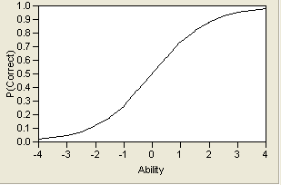
Of course, this is an unrealistic item, but it is illustrative in showing how a trait and a question probability relate to each other. More typical is a curve that allows probabilities that vary from zero to one. A typical curve found empirically is the S-shaped logistic function with a lower asymptote at zero and upper asymptote at one. It is markedly nonlinear. An example curve is shown in Example Item Response Curve.
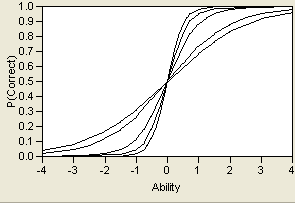
In this model, referred to as a Three-Parameter Logistic (3PL) model, the variable a represents the steepness of the curve at its inflection point. Curves with varying values of a are shown in Logistic Model for Several Values of a. This parameter can be interpreted as a measure of the discrimination of an item—that is, how much more difficult the item is for people with high levels of the trait than for those with low levels of the trait. Very large values of a make the model practically the step function shown in Item Characteristic Curve of a Perfect Scale Item. It is generally assumed that an examinee will have a higher probability of getting an item correct as their level of the trait increases. Therefore, a is assumed to be positive and the ICC is monotonically increasing. Some use this positive-increasing property of the curve as a test of the appropriateness of the item. Items whose curves do not have this shape should be considered as candidates to be dropped from the test.
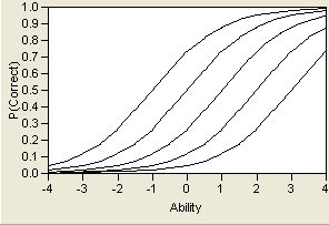
Changing the value of b merely shifts the curve from left to right, as shown in Logistic Curve for Several Values of b. It corresponds to the value of θ at the point where P(θ)=0.5. The parameter b can therefore be interpreted as item difficulty where (graphically), the more difficult items have their inflection points farther to the right along their x-coordinate.
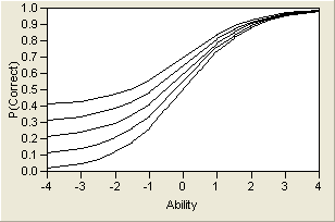
and therefore c represents the lower asymptote, which can be nonzero. ICCs for several values of c are shown graphically in Logistic Model for Several Values of c. The c parameter is theoretically pleasing, because a person with no ability of the trait might have a nonzero chance of getting an item right. Therefore, c is sometimes called the pseudo-guessing parameter.
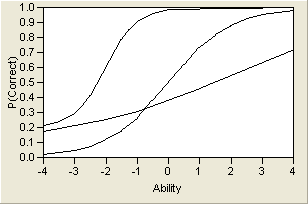
By varying these three parameters, a wide variety of probability curves are available for modeling. A sample of three different ICCs is shown in Three Item Characteristic Curves. Note that the lower asymptote varies, but the upper asymptote does not. This is because of the assumption that there might be a lower guessing parameter, but as the trait level increases, there is always a theoretical chance of 100% probability of correctly answering the item.
Note, however, that the 3PL model might by unnecessarily complex for many situations. If, for example, the c parameter is restricted to be zero (in practice, a reasonable restriction), there are fewer parameters to predict. This model, where only a and b parameters are estimated, is called the 2PL model.
Another advantage of the 2PL model (aside from its greater stability than the 3PL) is that b can be interpreted as the point where an examinee has a 50% chance of getting an item correct. This interpretation is not true for 3PL models.
A further restriction can be imposed on the general model when a researcher can assume that test items have equal discriminating power. In these cases, the parameter a is set equal to 1, leaving a single parameter to be estimated, the b parameter. This 1PL model is frequently called the Rasch model, named after Danish mathematician Georg Rasch, the developer of the model. The Rasch model is quite elegant, and is the least expensive to use computationally.
For example, open the sample data file MathScienceTest.jmp. These data are a subset of the data from the Third International Mathematics and Science Study (TIMMS) conducted in 1996.
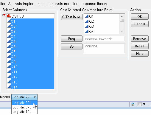
To launch the Item Analysis platform, select Analyze > Consumer Research > Item Analysis. This shows the dialog in Item Analysis Launch Window.
Specify the desired model (1PL, 2PL, or 3PL) by selecting it from the Model drop-down menu.
For this example, specify all fourteen continuous questions (Q1, Q2,..., Q14) as Y, Test Items and click OK. This accepts the default 2PL model.
If you select the 3PL model, a dialog pops up asking for a penalty for the c parameters (thresholds). This is not asking for the threshold itself. The penalty that it requests is similar to the type of penalty parameter that you would see in ridge regression, or in neural networks.
In cases where the items are questions on a multiple choice test where there are the same number of possible responses for each question, there is often reason to believe (a priori) that the threshold parameters would be similar across items. For example, if you are analyzing the results of a 20-question multiple choice test where each question had four possible responses, it is reasonable to believe that the guessing, or threshold, parameters would all be near 0.25. So, in some cases, applying a penalty like this has some “physical intuition” to support it, in addition to its computational advantages.

