The next sections give formulas for computing the least significant number (LSN), least significant value (LSV), power, and adjusted power. With the exception of LSV, these computations are provided for each effect, and for a collection of user-specified contrasts (under Custom Test and LS Means Contrast. LSV is only computed for a single linear contrast. In the details below, the hypothesis refers to the collection of contrasts of interest.
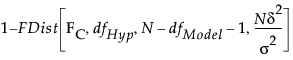
The LSN solves for N in the equation:
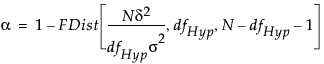
FDist is the cumulative distribution function of the central F distribution
dfHyp represents the degrees of freedom for the hypothesis
σ2 is the error variance
δ2 is the squared effect size
For retrospective analyses, δ2 is estimated by the sum of squares for the hypothesis divided by n, the size of the current sample. If the test is for an effect, then δ2is estimated by the sum of squares for that effect divided by the number of observations in the current study. For retrospective studies, the error variance σ2 is estimated by the mean square error. These estimates, along with an α value of 0.05, are entered into the Power Details window as default values.
When you are conducting a prospective analysis to plan a future study, consider determining the sample size that will achieve a specified power (see Computations for the Power.)
Consider the one-degree-freedom test Lβ = 0, where L is a row vector of constants. The test statistic for a t-test for this hypothesis is:
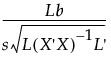
where s is the root mean square error. We reject the hypothesis at significance level α if the absolute value of the test statistic exceeds the 1 - α/2 quantile of the t distribution, t1-α/2, with degrees of freedom equal to those for error.
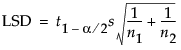
In the special case where the linear contrast tests a hypothesis setting a single βi equal to 0, this reduces to:
In a situation where the test of interest is a comparison of two group means, the literature talks about the least significant difference (LSD). In the special case where the model contains only one nominal variable, the formula for testing a single linear contrast reduces to the formula for the LSD:
Suppose that you are interested in computing the power of a test of a linear hypothesis, based on significance level α and a sample size of N. You want to detect an effect of size δ.
To calculate the power, begin by finding the critical value for an α-level F-test of the linear hypothesis. This is given by solving for FC in the equation
Here, dfHyp represents the degrees of freedom for the hypothesis, dfModel represents the degrees of freedom for the model, and N is the proposed (or actual) sample size.
Given an effect of size δ, the test statistic has a noncentral F distribution, with distribution function denoted FDist below, with noncentrality parameter λ. To obtain the power of your test, calculate the probability that the test statistic exceeds the critical value:
In obtaining retrospective power for a study with n observations, JMP estimates the noncentrality parameter λ = (nδ2)/σ2 by  , where SSHyp represents the sum of squares due to the hypothesis.
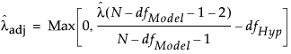
The estimate of the noncentrality parameter, λ, obtained by estimating δ and σ by their sample estimates, appears as follows:
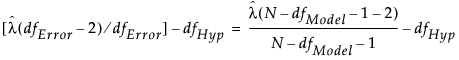
The expression on the right illustrates the calculation of the unbiased noncentrality parameter when a sample size N, different from the study size n, is proposed for a retrospective power analysis. Here, dfHyp represents the degrees of freedom for the hypothesis and dfModel represents the degrees of freedom for the whole model.