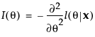
Consider first the case of a single parameter, θ. Let l be the log-likelihood function for θ and let x be the data. The score is the derivative of the log-likelihood function with respect to θ:

The score test can be generalized to multiple parameters. Consider the vector of parameters θ. Then the test statistic for the score test of H0:  is:
is:

The test statistic is asymptotically Chi-square distribution with k degrees of freedom. Here k is the number of unbounded parameters.
Let  be the value of
  where the algorithm terminates. Note that the relative gradient evaluated at
  is the score test statistic. A p-value is calculated using a Chi-square distribution with k degrees of freedom. This p-value gives an indication of whether the value of the unknown MLE is consistent with
  . The number of unbounded parameters listed in the Random Effects Covariance Parameter Estimates report equals k.
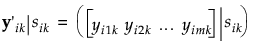
The standard random coefficient model specifies a random intercept and slope for each subject. Let yij denote the measurement of the jth observation on the ith subject. Then the random coefficient model can be written as follows:


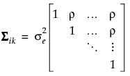
Assume that the sik are independent and identically distributed N(0, σs2) variables. Denote the number of treatment factors by t and the number of subjects by s. Then the distribution of eijk is N(0, Σ), where
Denote the block diagonal component of the covariance matrix Σ corresponding to the ikth subject within treatment by Σik. In other words, Σik = Var(yik|sik). Because observations over time within a subject are not typically independent, it is necessary to estimate the variance of yijk|sik. Failure to account for the correlation leads to distorted inference. The following sections describe the structures available for Σik.


Here tj is the time of observation j. In this structure, observations taken at any given time have the same variance,  . The parameter ρ, where -1 < ρ < 1, is the correlation between two observations that are one unit of time apart. As the time difference between observations increases, their covariance decreases because ρ is raised to a higher power. In many applications, AR(1) provides an adequate model of the within subject correlation, providing more power without sacrificing Type I error control.
|
•
|
|
•
|

 .
.Consider the simple model  . The spatial or temporal structure is modeled through the error term, ei. In general, the spatial correlation model can be defined as
  and
and .
.
Let si denote the location of yi, where si is specified by coordinates reflecting space or time. The spatial or temporal structure is typically restricted by assuming that the covariance is a function of the Euclidean distance, dij, between si and sj. The covariance can be written as  , where
  represents the correlation between observations yi and yj.
In the case of two or more location coordinates, if f(dij) does not depend on direction, then the covariance structure is isotropic. If it does, then the structure is anisotropic.
The correlation structures for spatial models available in JMP are shown below. These are parametrized by ρ, which is positive unless it is otherwise constrained.

|
•
|
|
•
|
When the spatial process is second-order stationary, the structures listed in Spatial Correlation Structures define variograms. Borrowed from geostatistics, the variogram is the standard tool for describing and estimating spatial variability. It measures spatial variability as a function of the distance, dij, between observations using the semivariance.
Let Z(s) denote the value of the response at a location s. The semivariance between observations at si and sj is given as follows:
If the process is isotropic, the semivariance depends only on the distance h between points and the function can be written as follows:
Defined as the value of the semivariogram at the plateau reached for larger distances. It corresponds to the variance of an observation. In models with no nugget effect, the sill is  . In models with a nugget effect, the sill is
  , where c1 represents the nugget. The partial sill is defined as
  .
.
Defined as the distance at which the semivariogram reaches the sill. At distances less than the range, observations are spatially correlated. For distances greater than or equal to the range, spatial correlation is effectively zero. In spherical models, ρ is the range. In exponential models, 3ρ is the practical range. In Gaussian models,  is the practical range. The practical range is defined as the distance where covariance is reduced to 95% of the sill.
In Fit a Spatial Structure Model, the repeated effects covariance parameter estimates represent the various semivariogram features:
For a given isotropic spatial structure, the estimated variogram is obtained using a nonlinear least squares fit of the observed data to the appropriate function in Spatial Correlation Structures.
To compute the empirical semivariance, the distances between all pairs of points for the variables selected for the variogram covariance are computed. The range of the distances is divided into 10 equal intervals. If the data do not allow for 10 intervals, then as many intervals as possible are constructed.
Distance classes consisting of pairs of points are constructed. The hth distance class consists of all pairs of points whose distances fall in the hth interval.
Ch
Z(x)
γ(h)
The semivariance function, γ, is defined as follows:
