To compute the pth quantile of n non-missing values in a column, arrange the n values in ascending order and call these column values y1, y2, ..., yn. Compute the rank number for the pth quantile as p / 100(n + 1).
|
•
|
If the result is an integer, the pth quantile is that rank’s corresponding value.
|
|
•
|
If the result is not an integer, the pth quantile is found by interpolation. The pth quantile, denoted qp, is computed as follows:
|
|
‒
|
n is the number of non-missing values for a variable
|
|
‒
|
|
‒
|
|
‒
|
|
‒
|
The value y12 is the 75th quantile. The 90th quantile is interpolated by computing a weighted average of the 14th and 15th ranked values as y90 = 0.6y14 + 0.4y15.
The mean is the sum of the non-missing values divided by the number of non-missing values. If you assigned a Weight or Freq variable, the mean is computed by JMP as follows:
The standard deviation measures the spread of a distribution around the mean. It is often denoted as s and is the square root of the sample variance, denoted s2.

The standard error means is computed by dividing the sample standard deviation, s, by the square root of N. In the launch window, if you specified a column for Weight or Freq, then the denominator is the square root of the sum of the weights or frequencies.
 where
where 

where wi is a weight term (= 1 for equally weighted items). Using this formula, the Normal distribution has a kurtosis of 0.
where ri is the rank of the ith observation, and N is the number of non-missing (and nonexcluded) observations.
where Φ is the cumulative probability distribution function for the normal distribution.
|
•
|
There are N observations:
|
|
•
|
The differences between observations and the hypothesized value m are calculated as follows:
|
|
•
|
There are N pairs of observations from two populations:
|
|
•
|
When there are tied absolute differences, they are assigned the average, or midrank, of the ranks of the observations.
|

R+ is the sum of the positive signed ranks
For  , exact p-values are calculated.
For N > 20, a Student’s t approximation to the statistic defined below is used. Note that a correction for ties is applied. See Iman (1974) and Lehmann (1998).

The last summation in the expression for Var(W) is a correction for ties. The notation di for i > 0 represents the number of values in the ith group of non-zero signed ranks. (If there are no ties for a given signed rank, then di = 1 and the summand is 0.)
The statistic t given by the following has an approximate t distribution with N - 1 degrees of freedom:

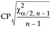
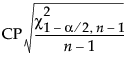
The Test Statistic is distributed as a Chi-square variable with n - 1 degrees of freedom when the population is normal.
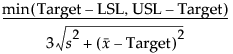
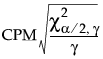
The Min PValue is the p-value of the two-tailed test, and is calculated as follows:
 where:
|
•
|
|
•
|
N is the number of non-missing observations
|
|
•
|
X is the original column
|
|
•
|
|
|
•
|
For m future observations:
|
|
•
|
For the mean of m future observations:
|
|
•
|
For the standard deviation of m future observations:
|
 for
for |
•
|
The one-sided intervals are formed by using 1-α in the quantile functions.
|
t is the quantile from the non-central t-distribution, and  is the standard normal quantile.
s = standard deviation and  is a constant that can be found in Table 4 of Odeh and Owen 1980).
To determine g, consider the fraction of the population captured by the tolerance interval. Tamhane and Dunlop (2000) give this fraction as follows:
where Φ denotes the standard normal c.d.f. (cumulative distribution function). Therefore, g solves the following equation:

where 1-γ is the fraction of all future observations contained in the tolerance interval.
|
•
|
Long-term uses the overall sigma. This option is used for
|

Note: There is a preference for Distribution called Ppk Capability Labeling that labels the long-term capability output with Ppk labels. This option is found using File > Preferences, then select Platforms > Distribution.
|
•
|
Specified Sigma enables you to type a specific, known sigma used for computing capability analyses. Sigma is user-specified, and is therefore not computed.
|
|
•
|
Moving Range enables you to enter a range span, which computes sigma as follows:
|
d2(n) is the expected value of the range of n independent normally distributed variables with unit standard deviation.
|
•
|
Short Term Sigma, Group by Fixed Subgroup Size if r is the number of subgroups of size nj and each ith subgroup is defined by the order of the data, sigma is computed as follows:
|
 where
where 
|
(USL - LSL)/6s where:
|
||
 |
||
 |
||
 |
||
 |
||
 |
||
 where γ = same as above.
|
||
 , where
|
•
|
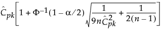
Exact 100(1 - α)% lower and upper confidence limits for CPL are computed using a generalization of the method of Chou et al. (1990), who point out that the 100(1 - α) lower confidence limit for CPL (denoted by CPLLCL) satisfies the following equation:
|
where Tn-1(δ) has a non-central t-distribution with n - 1 degrees of freedom and noncentrality parameter δ.
|
•
|
Exact 100(1 - α)% lower and upper confidence limits for CPU are also computed using a generalization of the method of Chou et al. (1990), who point out that the 100(1 - α) lower confidence limit for CPU (denoted CPULCL) satisfies the following equation:
|
where Tn-1(δ) has a non-central t-distribution with n - 1 degrees of freedom and noncentrality parameter δ.
For example, if there are 3 defects in n=1,000,000 observations, the formula yields 6.03, or a 6.03 sigma process. The results of the computations of the Sigma Quality Above USL and Sigma Quality Below LSL column values do not sum to the Sigma Quality Total Outside column value because calculating Sigma Quality involves finding normal distribution quantiles, and is therefore not additive.
The Normal fitting option estimates the parameters of the normal distribution. The normal distribution is often used to model measures that are symmetric with most of the values falling in the middle of the curve. Select the Normal fitting for any set of data and test how well a normal distribution fits your data.
|
•
|
μ (the mean) defines the location of the distribution on the x-axis
|
|
•
|
σ (standard deviation) defines the dispersion or spread of the distribution
|
The standard normal distribution occurs when  and
and  . The Parameter Estimates table shows estimates of μ and σ, with upper and lower 95% confidence limits.
pdf: 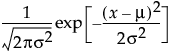 for
for  ;
;  ; 0 < σ
for The LogNormal fitting option estimates the parameters μ (scale) and σ (shape) for the two-parameter lognormal distribution. A variable Y is lognormal if and only if  is normal. The data must be greater than zero.
 for
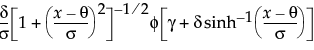
for The Weibull distribution has different shapes depending on the values of α (scale) and β (shape). It often provides a good model for estimating the length of life, especially for mechanical devices and in biology. The Weibull option is the same as the Weibull with threshold option, with a threshold (θ) parameter of zero. For the Weibull with threshold option, JMP estimates the threshold as the minimum value. If you know what the threshold should be, set it by using the Fix Parameters option. See Fit Distribution Options.
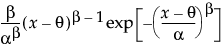 for
for 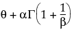

The Extreme Value distribution is a two parameter Weibull (α, β) distribution with the transformed parameters δ = 1 / β and λ = ln(α).
The Exponential distribution is a special case of the two-parameter Weibull when β = 1 and α = σ, and also a special case of the Gamma distribution when α = 1.
Devore (1995) notes that an exponential distribution is memoryless. Memoryless means that if you check a component after t hours and it is still working, the distribution of additional lifetime (the conditional probability of additional life given that the component has lived until t) is the same as the original distribution.
The Gamma fitting option estimates the gamma distribution parameters, α > 0 and σ > 0. The parameter α, called alpha in the fitted gamma report, describes shape or curvature. The parameter σ, called sigma, is the scale parameter of the distribution. A third parameter, θ, called the Threshold, is the lower endpoint parameter. It is set to zero by default, unless there are negative values. You can also set its value by using the Fix Parameters option. See Fit Distribution Options.
|
•
|
The standard gamma distribution has σ = 1. Sigma is called the scale parameter because values other than 1 stretch or compress the distribution along the x-axis.
|
|
•
|
|
•
|
The standard beta distribution is useful for modeling the behavior of random variables that are constrained to fall in the interval 0,1. For example, proportions always fall between 0 and 1. The Beta fitting option estimates two shape parameters, α > 0 and β > 0. There are also θ and σ, which are used to define the lower threshold as θ, and the upper threshold as θ + σ. The beta distribution has values only for the interval defined by 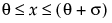 . The θ is estimated as the minimum value, and σ is estimated as the range. The standard beta distribution occurs when θ = 0 and σ = 1.
Set parameters to fixed values by using the Fix Parameters option. The upper threshold must be greater than or equal to the maximum data value, and the lower threshold must be less than or equal to the minimum data value. For details about the Fix Parameters option, see Fit Distribution Options.
The Normal Mixtures option fits a mixture of normal distributions. This flexible distribution is capable of fitting multi-modal data.
Fit a mixture of two or three normal distributions by selecting the Normal 2 Mixture or Normal 3 Mixture options. Alternatively, you can fit a mixture of k normal distributions by selecting the Other option. A separate mean, standard deviation, and proportion of the whole is estimated for each group.


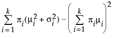
where μi, σi, and πi are the respective mean, standard deviation, and proportion for the ith group, and  is the standard normal pdf.
The Smooth Curve option fits a smooth curve using nonparametric density estimation (kernel density estimation). The smooth curve is overlaid on the histogram and a slider appears beneath the plot. Control the amount of smoothing by changing the kernel standard deviation with the slider. The initial Kernel Std estimate is calculated from the standard deviation of the data.
 for
for  for
for  for
for
Note: The parameter confidence intervals are hidden in the default report. Parameter confidence intervals are not very meaningful for Johnson distributions, because they are transformations to normality. To show parameter confidence intervals, right-click in the report and select Columns > Lower 95% and Upper 95%.
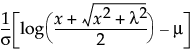
This distribution is useful for fitting data that are rarely normally distributed and often have non-constant variance, like biological assay data. The Glog distribution is described with the parameters μ (location), σ (scale), and λ (shape).
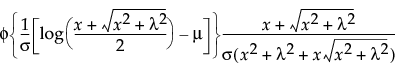
 ~ N(0,1), then
Note: The parameter confidence intervals are hidden in the default report. Parameter confidence intervals are not very meaningful for the GLog distribution, because it is a transformation to normality. To show parameter confidence intervals, right-click in the report and select Columns > Lower 95% and Upper 95%.
In the Compare Distributions report, the ShowDistribution list is sorted by AICc in ascending order.
|
‒
|
n is the sample size
|
|
‒
|
ν is the number of parameters
|
pmf:  for
for  ; x = 0,1,2,...
This distribution is useful when the data is a combination of several Poisson(μ) distributions, each with a different μ. One example is the overall number of accidents combined from multiple intersections, when the mean number of accidents (μ) varies between the intersections.
The Gamma Poisson distribution results from assuming that x|μ follows a Poisson distribution and μ follows a Gamma(α,τ). The Gamma Poisson has parameters λ = ατ and σ = τ+1. The parameter σ is a dispersion parameter. If σ > 1, there is over dispersion, meaning there is more variation in x than explained by the Poisson alone. If σ = 1, x reduces to Poisson(λ).
pmf: 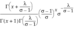 for
for  ;
;  ; x = 0,1,2,...
for Remember that x|μ ~ Poisson(μ), while μ~ Gamma(α,τ). The platform estimates λ = ατ and σ = τ+1. To obtain estimates for α and τ, use the following formulas:

If the estimate of σ is 1, the formulas do not work. In that case, the Gamma Poisson has reduced to the Poisson(λ), and  is the estimate of λ.
If the estimate for α is an integer, the Gamma Poisson is equivalent to a Negative Binomial with the following pmf:
Run demoGammaPoisson.jsl in the JMP Samples/Scripts folder to compare a Gamma Poisson distribution with parameters λ and σ to a Poisson distribution with parameter λ.
The Binomial option accepts data in two formats: a constant sample size, or a column containing sample sizes.
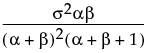
The Beta Binomial distribution results from assuming that x|π follows a Binomial(n,π) distribution and π follows a Beta(α,β). The Beta Binomial has parameters p = α/(α+β) and δ = 1/(α+β+1). The parameter δ is a dispersion parameter. When δ > 0, there is over dispersion, meaning there is more variation in x than explained by the Binomial alone. When δ < 0, there is under dispersion. When δ = 0, x is distributed as Binomial(n,p). The Beta Binomial only exists when  .
.

Remember that x|π ~ Binomial(n,π), while π ~ Beta(α,β). The parameters p = α/(α+β) and δ = 1/(α+β+1) are estimated by the platform. To obtain estimates of α and β, use the following formulas:


If the estimate of δ is 0, the formulas do not work. In that case, the Beta Binomial has reduced to the Binomial(n,p), and  is the estimate of p.
Run demoBetaBinomial.jsl in the JMP Samples/Scripts folder to compare a Beta Binomial distribution with dispersion parameter δ to a Binomial distribution with parameters p and n = 20.
The fitted quantiles in the Diagnostic Plot and the fitted quantiles saved with the Save Fitted Quantiles command are formed using the following method:
|
2.
|
|
3.
|
Compute the quantile[i] = Quantiled(p[i]) where Quantiled is the quantile function for the specific fitted distribution, and i = 1,2,...,n.
|
|
μ and σ are unknown
|
Shapiro-Wilk (for n ≤ 2000) Kolmogorov-Smirnov-Lillefors (for n > 2000)
|
|
|
μ and σ are both known
|
||
|
μ and σ are known or unknown
|
||
|
α and β known or unknown
|
||
|
α and β known or unknown
|
||
|
σ is known or unknown
|
||
|
α and σ are known
|
||
|
α and β are known
|
||
|
ρ is known or unknown and n is known
|
||
|
ρ and δ known or unknown
|
||
|
λ known or unknown
|
||
|
λ or σ known or unknown
|
Writing T for the target, LSL, and USL for the lower and upper specification limits, and Pα for the α*100th percentile, the generalized capability indices are as follows:


If the data are normally distributed, these formulas reduce to the formulas for standard capability indices. See Descriptions of Capability Indices and Computational Formulas.
Type a K value and select one-sided or two-sided for your capability analysis. Tail probabilities corresponding to K standard deviations are computed from the Normal distribution. The probabilities are converted to quantiles for the specific distribution that you have fitted. The resulting quantiles are used for specification limits in the capability analysis. This option is similar to the Quantiles option, but you provide K instead of probabilities. K corresponds to the number of standard deviations that the specification limits are away from the mean.
For example, for a Normal distribution, where K=3, the 3 standard deviations below and above the mean correspond to the 0.00135th quantile and 0.99865th quantile, respectively. The lower specification limit is set at the 0.00135th quantile, and the upper specification limit is set at the 0.99865th quantile of the fitted distribution. A capability analysis is returned based on those specification limits.