"That figure is wrong," someone in the audience said at a recent JMP demo when I showed a capability plot similar to the first figure below, with the spec limits at ±6σ from the mean. In their view, the spec limits should be at ±3σ. I am assuming they thought that the “six” in “Six Sigma” comes from adding up 3σ on either side of the mean. Actually, the figure is correct. And while those six standard deviations do explain the name “Six Sigma,” there's more to the story than that.

Why Six Sigma isn’t really ±6σ (and why that’s the point)

If you’ve ever taken a Six Sigma class, or taught one, as I have, there’s a moment where things stop quite making sense. You learn that Six Sigma means six standard deviations on either side of the mean. You also learn that a Six Sigma process is famous for one particular number: 3.4 defects per million opportunities (DPMO). But when you use a Z score to calculate the probability associated with 6σ from the mean, the result is only about 0.001 parts per million in each tail, or roughly 2 defects per billion.

We can show this visually using JMP’s interactive capability plot, shown in Figure 1 below. With an upper specification limit (USL)=34, lower specification limit (LSL)=10, Mean (m)=22, and sample standard deviation of 2, the specification limits are exactly 6σ from the mean. Circled on the right is the output for a Six Sigma process where 0.001 ppm are the expected defects outside the upper spec limit and 0.001 ppm are the expected defects on the lower side.

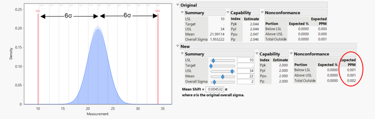
So the math says a Six Sigma process results in an expected defect rate of 2 defects per billion, yet Six Sigma is famously associated with 3.4 defects per million, a rate about 1,000 times higher. The 3.4 DPMO figure is actually closer to a 4.5σ process. So, what’s going on?

Statistically ideal: A perfectly centered process

In pure statistics, the definition is straightforward. Assuming a process is normally distributed, perfectly centered, and stable over time, then:

• ±3σ captures 99.73% of outcomes.

• ±6σ captures virtually everything.

At ±6σ, defect rates are very small, almost theoretical. If the world behaved like a textbook, we’d stop right here. But it doesn’t.

The reality: Processes drift

Real-world processes don’t stay centered. Over time, machines wear down, materials vary, operators change, and environments shift. And most importantly: the process mean moves.

At Motorola, where the Six Sigma methodology was first introduced in the 1980s, the company studied this extensively and found that even well-controlled processes tend to drift over time. This phenomenon was dubbed long-term dynamic mean variation. And this insight changed everything.

The 1.5 Sigma shift

Rather than ignore this reality, Motorola did something bold: it built it into the definition of Six Sigma. Based on empirical data, its engineers observed that the process mean typically shifts by about 1.5 standard deviations over time. This is what’s known as the 1.5σ shift. It represents the gap between:

• Short-term performance (what you measure in a study).

• Long-term performance (what your customer actually experiences).

From 6 Sigma to 4.5 Sigma

Now let’s connect the dots. Start with a perfectly centered process:

• Distance to spec limits = 6σ

Now apply real-world drift:

• Mean shifts 1.5σ toward the upper spec limit.

The effective distance becomes: 6σ – 1.5σ = 4.5σ.

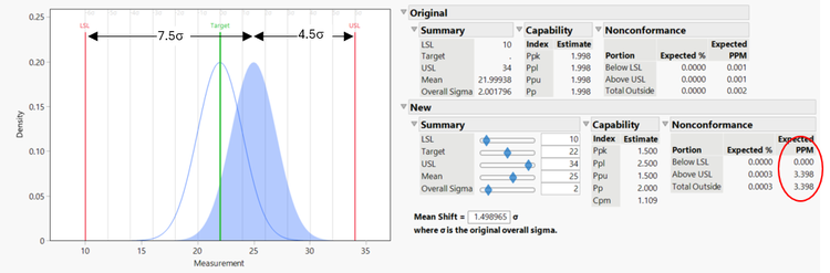
Referring to JMP’s interactive capability plot shown in Figure 2 below, the process has moved or shifted by 1.5σ to the right, and the process is no longer centered. It shifts the process upward, creating more defects outside of the USL. Circled in red is approximately how many defects per million parts would be created, which is where the famous 3.4 ppm for a Six Sigma process comes from. But now, we know this is actually for a 4.5 Sigma process, not a Six Sigma process.

Two definitions, one concept

This distinction leads to one of the most important (and most misunderstood) insights in Six Sigma:

Six Sigma actually has two meanings

Why not just call it 4.5 Sigma?

This is where the philosophy comes in. If your process only operates at 4.5σ under ideal conditions, then after the inevitable process drift, you’re no longer capable.

Six Sigma flips that thinking: design the process to be 6σ capable so that even after it drifts, it still performs at a high level. It’s not about perfection. It’s about robustness.

To understand why Six Sigma represented such a dramatic change in thinking, compare it to the traditional 3σ benchmark: a 3σ process, subject to the same 1.5σ drift, produces 66,807 defects per million.

That might sound like “good quality” until you translate it into actual consequences: thousands of failures, significant rework, and customer dissatisfaction. Six Sigma marked a shift in mindset from “acceptable defects” to “engineered reliability.

A different way to think about it

A useful analogy is engineering design. Designing for 3σ is like designing a bridge for average traffic. Designing for 6σ is designing for worst-case conditions – weather, load, aging, etc.

And the 1.5σ shift? That’s the assumption that conditions will change. Because they always do.

The controversy (and the truth)

It’s worth noting that the 1.5σ shift is not a universal statistical law. It’s an empirical convention based on Motorola’s observations. Some industries with tightly controlled processes (pharmaceutical, for example) experience less drift. Other industries with complex manufacturing systems experience more drift.

The amount of drift varies, but short-term data tends to overestimate long-term performance.

Final takeaway

Six Sigma isn’t just about six standard deviations. It’s about designing processes that remain capable, even when reality interferes. A clean way to say it:

Six Sigma is not six standard deviations from failure. It’s six standard deviations from failure – even after your process starts to drift.