Penalized Regression
What is penalized regression?
Penalized regression is a family of regression methods that modifies ordinary least squares (OLS) regression by adding a penalty in the fitting process. Like linear regression, the goal is to find coefficient estimates that describe the relationship between a response and predictors. Unlike linear regression, the method does not minimize the sum of squared errors; it minimizes the sum of squared errors plus a penalty. Different methods use different penalties. Using a penalty results in shrinkage of coefficients, so these methods are sometimes called shrinkage methods. Penalized regression models are especially useful for situations where predictors are correlated, or when your goal is model term selection.
How does penalized regression reduce variance?
Penalized regression estimators and predictions tend to have lower variance than those of ordinary least squares regression. To get the lower variance, penalized regression gives up the unbiasedness that OLS offers. The goal is variance reduction while introducing only a small increase in bias.
How to think about bias
Ordinary least squares regression gives unbiased estimates of the regression parameters under the usual model assumptions. It means that if you were to sample from the population many times, fit the regression model many times, then average the coefficients over the samples, the average would be very close to the true value of the coefficient. In contrast, the penalized regression estimators of the parameters are biased, and the average would be farther from the true value.
How to think about variance of estimates
OLS can suffer from large variance if the predictor variables are correlated, which means that if you were to sample from the population many times, the coefficients from the models would be quite different from each other. Penalized regression can lower the variance and give stability to both the estimates of coefficients and predictions. The procedure does so by giving up the unbiasedness of the estimators.
In the figure below, you can see that distribution of the OLS estimator (blue normal curve) is centered at the true value of the parameter, but it can have large variance. The penalized estimator distribution (purple normal curve) is centered slightly away from the true value, but its variance is much smaller.
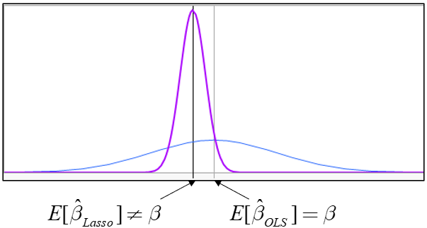
To see if the increase in bias is offset by the decrease in variance, you can use the mean squared error (MSE) of the regression parameters or the mean squared prediction error (MSPE) to measure both the bias and the variance at the same time. The MSE is the squared bias plus the variance of the estimator. The MSPE is the squared bias plus the variance of predictions. When comparing models, you might choose the model with the lower MSE or MSPE so that the reduction in variance more than offsets the increase in bias.
What is LASSO regression?
The least absolute shrinkage and selection operator, or LASSO, is a penalized regression method that can shrink some coefficient estimates exactly to zero. Because coefficients can be set to zero, LASSO can perform variable selection while fitting the model.
Like other penalized regression methods, LASSO finds the parameter estimates that minimize the sum of squared errors plus a penalty. The LASSO penalty is based on the sum of the absolute values of the coefficients. A tuning parameter controls the size of the penalty. When the penalty is large, coefficient estimates are pulled strongly toward zero. When the penalty is small, the fit approaches ordinary least squares for models where OLS can be fit.
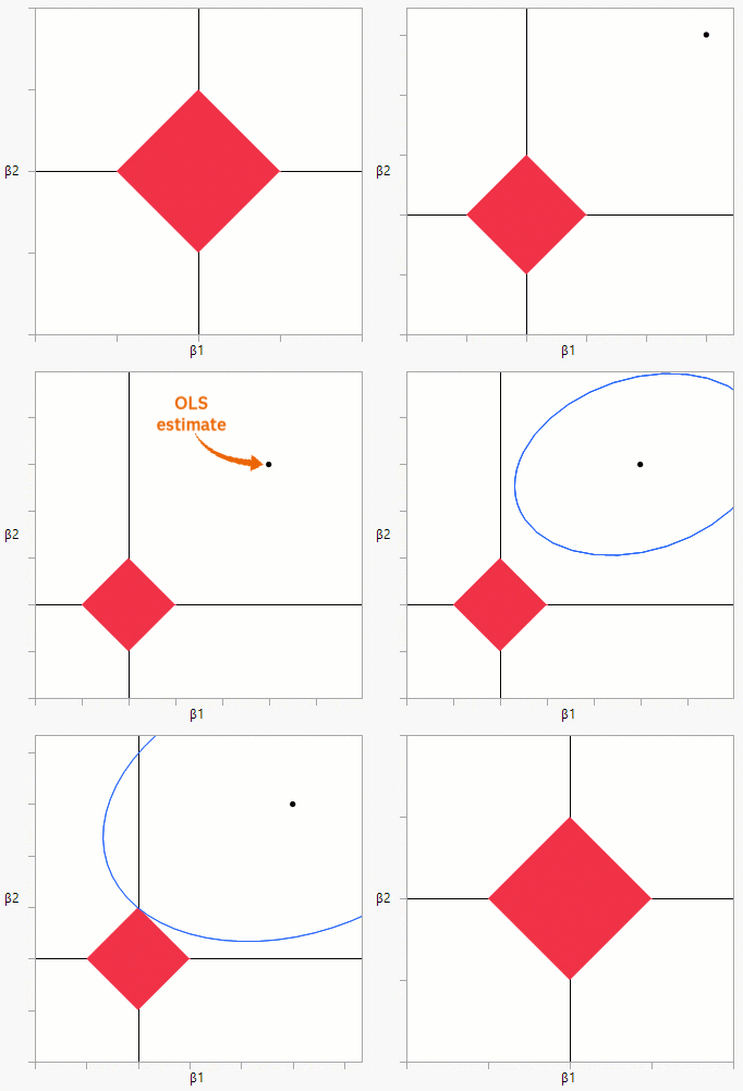
A geometric view helps explain why LASSO can select variables. With two predictors, the LASSO constraint forms a diamond-shaped region. In the figure below, the red diamond represents the penalty region. The LASSO estimate of ($\beta_1$, $\beta_2$) must lie in the penalty region. The black marker in the upper-right quadrant represents the OLS estimate ($\hat\beta_1$, $\hat\beta_2$) of the two coefficients, which lies outside the penalty region. The blue ellipse represents a contour of the least squares error function (the sum of squared errors). All values of $\beta_1$ and $\beta_2$ on the ellipse have the same value of the error function. The OLS solution minimizes the least squares error function; it’s at the center of the ellipse.
As the ellipse gets bigger, the sum of squared errors is no longer minimized – it is getting bigger. The LASSO solution must be within the red diamond. The first point where the ellipse intersects the diamond is the point with the least sum of squared errors that also satisfies the constraint.
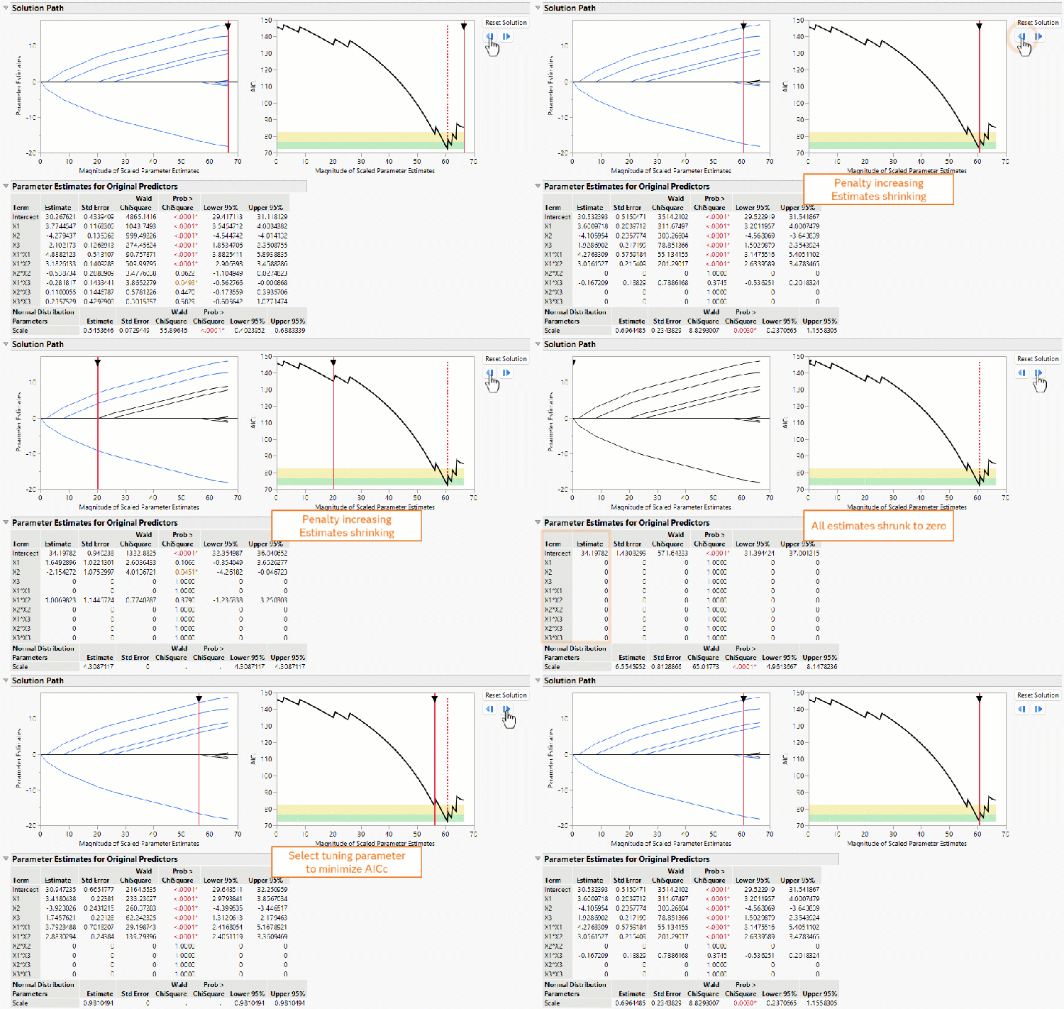
The LASSO solution path, shown in the left graph in the figure below, plots how the coefficient estimates change as the penalty tuning parameter changes. Each blue curve represents the path of the parameter estimate for one term in the model. On the left of the X axis, the tuning parameter is large and most coefficients are zero. At the other end, the tuning parameter is small, and more predictors can enter the model. You can think about the right side of this graph as showing the OLS estimates. You can see how the estimates shrink to zero as you travel left, increasing the penalty. The vertical red line is drawn at an optimal value of the tuning parameter, chosen by AICc.
Model selection criteria such as AICc can be used to choose the value of the penalty tuning parameter. The graph on the right in the figure below shows the value of AICc as the tuning parameter changes. Note that both these graphs have the same X axis values, so as you move the red line in one, it moves in the other. The optimal value of the tuning parameter minimizes this AICc curve. For an explanation of AICc as a model comparison criterion, see A Deeper Dive into Likelihood - JMP User Community.

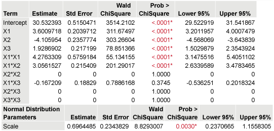
Numeric output for a LASSO model, shown in the table below, typically includes coefficient estimates, standard errors, and hypothesis tests. Predictors with estimates of zero have been removed from the model. The final line in the table is an estimate of the standard deviation of the errors. It corresponds to the RMSE of ordinary regression. Because the same data are being used for model selection and model evaluation, hypothesis tests and confidence intervals should be interpreted with care.
When should I use LASSO regression?
Use LASSO regression when you have many possible predictors and want the model to identify a smaller set of important variables. LASSO is especially useful when you expect only some predictors to have meaningful effects, that is, when you have sparsity of effects.
Use caution when predictors are highly correlated. In that situation, LASSO might choose just one predictor from a group and set the other coefficients to zero, even when several predictors contain similar information and thus explain variability in the response. For example, in a health study, three separate variables measure a patient’s cholesterol. These variables are highly correlated. LASSO might select only one variable. Other penalized methods, such as ridge or elastic net regression, might include all three correlated variables in the model.
What is ridge regression?
Ridge regression is another penalized regression method that was originally developed to solve the problem of collinearity in the predictors. Instead of penalizing the sum of the absolute values of the coefficients as in LASSO, ridge regression penalizes the sum of squared coefficient values. This penalty shrinks coefficients toward zero, but it generally does not set coefficients exactly to zero.
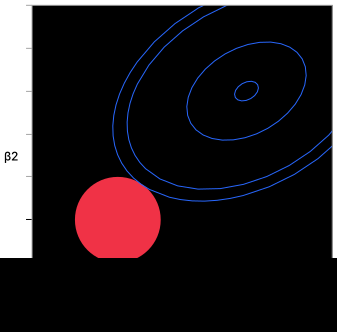
The ridge penalty produces a circular constrained region in the two-predictor case, seen below. With more than two predictors, the region is a hypersphere. Because the constraint has no corners, the solution does not usually land on an axis. As a result, ridge regression is not a variable selection method. Instead, it is used to reduce the variance caused by the correlation among predictors. There is still a corresponding increase in bias, but the hope is that it will be overcome by the decrease in variance.
When should I use ridge regression?
Use ridge regression when predictors are correlated and you want more stable coefficient estimates and predictions than ordinary least squares regression. Collinearity among the predictors inflates the variance of the parameter estimates and predictions. Penalizing the error function with the sum of squared coefficients reduces the variance.
What is elastic net regression?
Elastic net regression combines the LASSO and ridge penalties. One tuning parameter controls the overall amount of shrinkage, and another controls the balance between the LASSO penalty and the ridge penalty. It makes elastic net useful when you want variable selection but also expect groups of correlated predictors. Elastic net can overcome some limitations of LASSO. When predictors are highly correlated, LASSO might select only one predictor from a group. Elastic net tends to keep related predictors together while still allowing variable selection by shrinking some coefficients to zero.
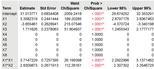
The graphical output of the elastic net is similar to that of the LASSO. The solution path and parameter estimates are shown below.

When should I use elastic net regression?
The elastic net model is useful when you have sparse effects (same as LASSO) or correlated predictors (same as ridge regression).
What are adaptive methods?
Adaptive methods recognize that if a predictor has a large OLS estimate, it is likely to be an active factor. The penalty is decreased proportionally to the OLS estimate, which means that different predictors are penalized by different amounts. Predictors with stronger initial evidence of an effect receive a smaller penalty, while predictors with weaker evidence receive a larger penalty. The goal is to improve variable selection by making it easier to keep potential active factors in the model.
The adaptive LASSO and adaptive elastic net have the oracle property: as sample size increases, the probability that the correct model is chosen approaches 1. Also, as sample size increases, the variance of the estimates of the nonzero predictors approaches the same variance as the OLS estimates.
When should I use adaptive methods?
Use adaptive methods when you want variable selection that can give stronger predictors more opportunity to remain in the model. These methods can be helpful when there is enough data to support reliable initial estimates and when the goal is to identify an interpretable set of active predictors. Adaptive methods can fail when the sample size is small or when predictors are strongly correlated.