SHASH Distribution
What is the SHASH distribution?
The SHASH distribution (short for sinh-arcsinh) is a continuous probability distribution that can model data with skewness, unusual tail behavior, or both. It has four parameters: location, scale, skewness, and tail weight. When the skewness parameter $\gamma$ = 0 and the tail-weight parameter $\delta$ = 1, the SHASH distribution becomes a normal distribution.
What are some examples of the SHASH distribution?
Examples of data that a SHASH distribution might describe include:
- Daily rainfall or other environmental measurements with many small values and a few large values.
- Measurements with heavier or lighter tails than a normal distribution.
- Continuous data whose shape cannot be captured well by a familiar symmetric distribution.
When should I consider using the SHASH distribution?
Consider the SHASH distribution when your data are continuous and a normal distribution does not fit because the data are asymmetric or have unusually light or heavy tails. Like the Johnson family, SHASH is flexible enough to represent many combinations of mean, variance, skewness, and kurtosis. It is especially useful when you want one model that can adjust both asymmetry and tail behavior.
What are the characteristics of the SHASH distribution?
The SHASH distribution is created by transforming a standard normal random variable $Z$: The parameters $\mu$ and $\sigma$ control location and scale, while $\gamma$ and $\delta$ control skewness and tail weight.
SHASH is a mathematically constructed distribution rather than a model derived from a specific physical process. Its flexibility makes it useful for describing many data shapes.
| Model parameters |
$\theta$, location $\sigma$, scale $\gamma$, shape, skewness $\delta$, shape, tail weight |
| Density function |
$f(x)=\frac{\delta \cosh(w)}{\sqrt{\sigma^2+(x-\theta)^2}}\,\phi(\sinh(w)),\;-\infty<x<\infty,\;-\infty<\gamma,\theta<\infty,\;\sigma,\delta>0$, where $\phi$ is the standard normal pdf and $w=\gamma+\delta\,\sinh^{-1}\!\left(\frac{x-\theta}{\sigma}\right)$ |
| Mean | no closed form expression |
| Variance | no closed form expression |
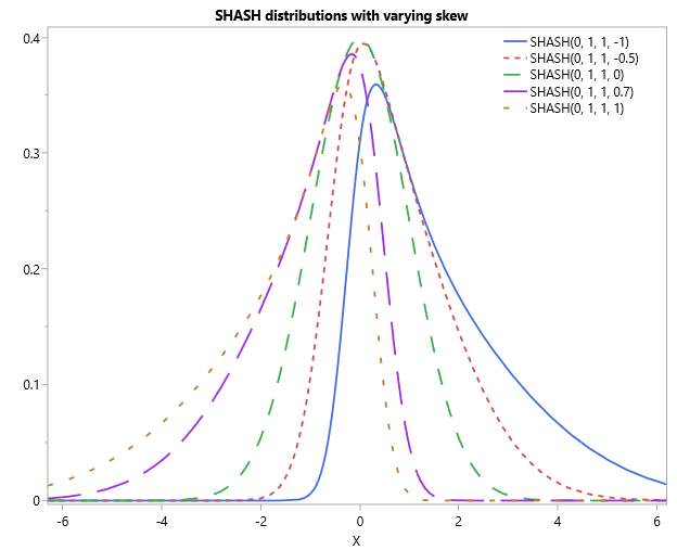
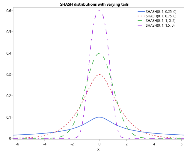
The graphs below show how changing the skewness or tail-weight parameter changes the shape of a SHASH distribution with the same location and scale parameters.
Example of a SHASH random variable
Suppose daily rainfall in an ecosystem follows a SHASH distribution with $\gamma$ = –8, $\delta$ = 5, $\mu$ = –2.9, and $\sigma$ = 2. What is the probability that a randomly chosen day has less than 1 mm of rainfall?
We use statistical software, like JMP, to evaluate the cumulative probability at 1 mm. In the JMP Scripting Language,
SHASH Distribution( 1, -8, 5, -2.9, 2 ) returns 0.154. Therefore, the probability of less than 1 mm of rainfall is 0.154, or 15.4%.