- JMP User Community
- :
- Learn JMP
- :
- Mastering JMP
- :
- Producing and Interpreting Basic Statistics
Practice JMP using these webinar videos and resources. We hold live Mastering JMP Zoom webinars with Q&A most Fridays at 2 pm US Eastern Time. See the list and register. Local-language live Zoom webinars occur in the UK, Western Europe and Asia. See your country jmp.com/mastering site.
- Subscribe to RSS Feed
- Mark as New
- Mark as Read
- Bookmark
- Subscribe
- Printer Friendly Page
- Report Inappropriate Content
See how to:
- Look at box plots and statistics, as originally proposed by Mary Eleanor Spear as a way to present information about populations of people
- Examine how box plots graphically communicate information about the central tendency and spread of data regardless of its underlying distribution
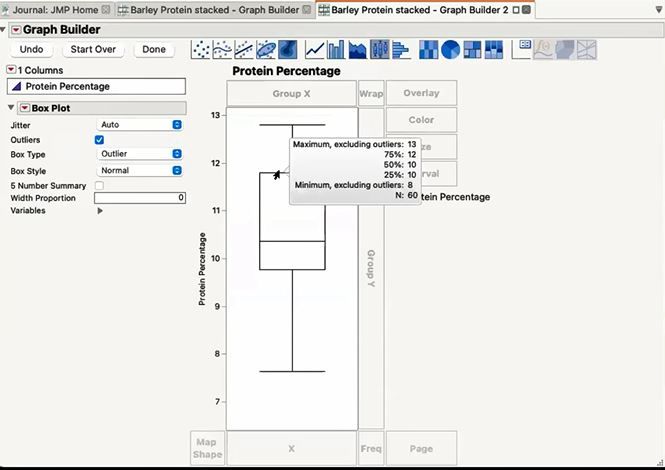
- Deploy JMP to create box plot to understand the distribution of the data and generate some statistics for Barley Protein data
-
Interpret JMP 16 and later Notched Box Plots, where JMP uses a horizontal line for the median rather than a notch and adds a mean diamond for the mean too.
- Use Student's t-test, as first presented by Sealy Gosset, to determine if a mean is different from a target or if two means are statistically the same, for example, if grain samples from different lots have the same (acceptable) protein content as a target value
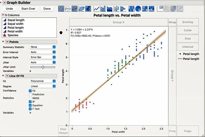
- Perform Exploratory Data Analysis (EDA), as codified and refined by John Tukey, to look at data that have potential relationships and examine some statistics that help understand the relationships


Resources
- Box Plots
- JMP Statistics Knowledge Portal - free online course in basic stats
- Mark as Read
- Mark as New
- Bookmark
- Get Direct Link
- Report Inappropriate Content
Hello JMP User Community
Thank you to @gail_massari , @MikeD_Anderson for hosting the Oct15-2021 Mastering JMP session, Producing and Interpreting Basic Statistics.
The "notched" Box Plots feature which you demoed, available in graph builder by right-clicking, is as super cool (and useful) feature!
During the session, several questions came up about hypothesis testing and the correct/meaningful interpretation of p-values in the context of hypothesis testing. For starters, I wanted to state that hypothesis testing is a normative prescriptive framework for optimal decisions under uncertainty, based on an instantiation of Occam's Razor (click on the links I cite below). Sampling error is the simplest (most parsimonious) explanation for explaining no treatment effect (the situation we are in under the null hypothesis), where sampling error is always present - this is just the inherent variation we get when taking repeated samples from a population.
A p-value is simply the proportion of area in a distribution under the null hypothesis, where that proportion (area covered) is just a probability.
Formally, in the framework of hypothesis testing, a p-value is the probability of obtaining a statistic (or more extreme) if the null hypothesis is true.
If the probability is "Low" then we have reason to reject the null hypothesis.
If the probability is "High" then we do not have reason to reject the null hypothesis.
Q. What determines whether the probability is "High" or "Low"? A. The criteria that we establish, usually before running an experiment.
What is that criteria? That criteria is simply a cut-off value, wherein we decide what that cut-off should be, and where that cut-off is customarily set at = 0.05 (or 5% as a general rule-of-thumb).
What do we call this criteria? Formally this cut-off is called "alpha" (α), otherwise known as our "standard of evidence."
If p is < α, then we reject the null hypothesis.
If p is ≥ α, then we do not reject the null hypothesis.
The null hypothesis is never accepted! Why? Lack of evidence of an effect in a particular experiment (in other words, p ≥ α) in no way serves as evidence that the effect is absent in the population. In Science or Industrial Experimentation we "keep looking". Especially if our sample size is small and/or we discover that our experimental results cannot be replicated. In Statistics, we usually consider a rejection statement on the null (p < α) much "stronger" evidence than a non-rejection statement (p is ≥ α). A "do not reject the null hypothesis" decision is in-effect a "we didn't find anything" decision. It doesn't prove that nothing is out there. If we assumed it did, then we wouldn't be doing Science or Industrial Experimentation (Life would be very boring).
Julian Parris (@julian) provides an outstanding treatment on the logic and framework of hypothesis testing in his (2015) JMP-driven statistics course Significantly Statistical Methods,
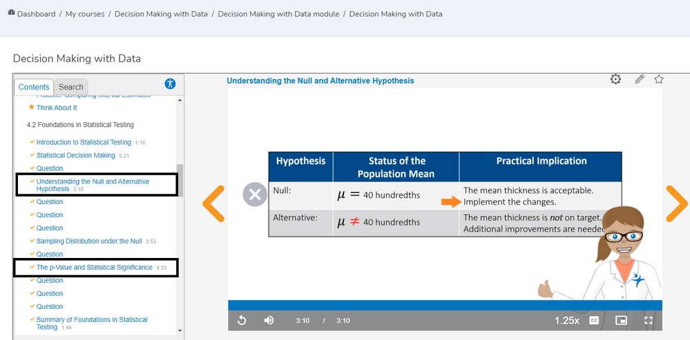
Hypothesis testing and p-values are also very well covered in the JMP STIPS module: Decision Making with Data, available in the SAS Virtual Learning Environment (and free of charge with the registration of a SAS username and password).
See Section 4.2 Foundations in Statistical Testing ("Understanding the Null and Alternative Hypothesis," and "The p-Value and Statistical Significance")
Hope this is helpful!
Recommended Articles
- © 2024 JMP Statistical Discovery LLC. All Rights Reserved.
- Terms of Use
- Privacy Statement
- About JMP
- JMP Software
- JMP User Community
- Contact

