Importing Data from IDAT Files
The IDAT file format is used to store BeadArray data generated by analysis systems from Illumina Inc. IDAT files are output directly from Illumina scanners in a proprietary format and store summary intensities for each probeset on an array in a compressed manner. IDAT files are not readable by text editors or other readily available software and scientists have been limited to using Illumina's software to extract and view the data.
With the release of version 17, JMP PRO is now able to open one or more IDAT files and combine them into a JMP table.
In this example, we import two IDAT files, GSM2277217_7973201017_R01C01_Grn.idat and GSM2277217_7973201017_R01C01_Red.idat, that were downloaded from GEO. These files contain data from an experiment comparing gene expression from methylated (red) or unmethylated (Green) loci. We import the data, perform preliminary analysis and quality control and normalization, and reformat them table for analysis. A zip file containing these files is available here for you to download.
Importing IDAT Files into JMP PRO
| 8 | Open JMP PRO. |
| 8 | Select File > Import Multiple Files.... |
| 8 | Navigate to the location of the files to be imported. |
| 8 | Check the Select Files by name or extension box. |
| 8 | Click and select .idat from the drop-down list. |
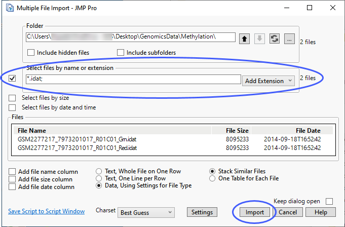
| 8 | Click . |
| 8 | You can specify a table containing annotation information if one is available. Otherwise, click to generate the JMP table. |
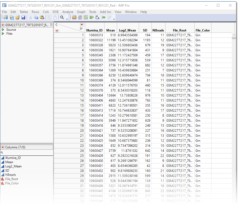
The resulting JMP table is a tall![]() A data table in which variables in rows and samples are in the columns table with probe sets making up the rows. It is a stacked table, with the contents of the second IDAT data set appended to the bottom of the first data set for a total of 1,244,798 rows. This table requires modification before we can use it for analysis in JMP.
A data table in which variables in rows and samples are in the columns table with probe sets making up the rows. It is a stacked table, with the contents of the second IDAT data set appended to the bottom of the first data set for a total of 1,244,798 rows. This table requires modification before we can use it for analysis in JMP.
Preliminary Analysis, Quantity Control, and Normalization
Although we have imported the data into JMP, the table requires some modification before we can use it for data analysis. Let us examine the data using JMPs Fit Y by X platform.
| 8 | Select Analyze > Fit Y by X. |
| 8 | Specify Log2_Mean as the Y, Response and File_Color as the X, Factor. |
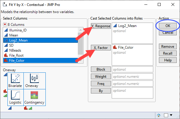
| 8 | Click . |
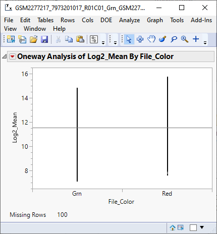
The one-way analysis (below) shows that the response means of the red and green samples are slightly shifted, relative to each other.
| 8 | Click  and select Densities > Compare Densities to compare the densities of the data from the two samples. and select Densities > Compare Densities to compare the densities of the data from the two samples. |
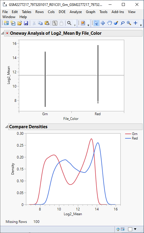
The density plot shows that density pattern of the two samples, while shifted, are very similar, indicating that normalizing the means should make direct comparisons between the two samples meaningful.
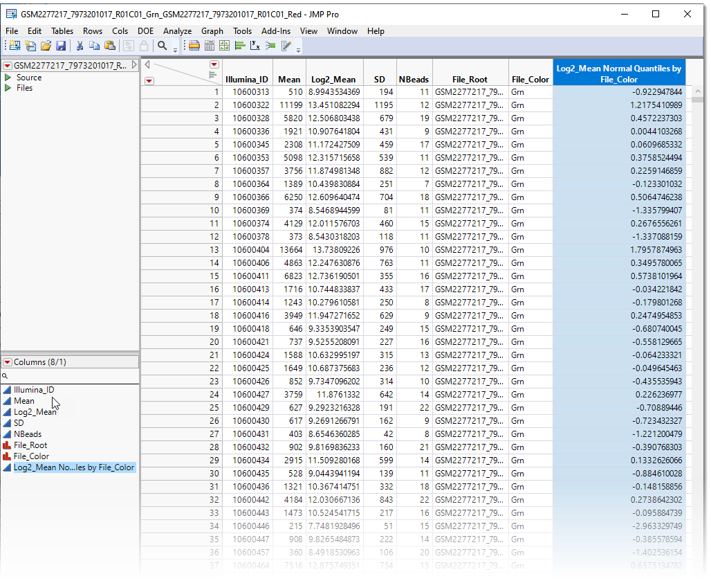
| 8 | Click  and select Save > Save Normal Quantiles and select Save > Save Normal Quantiles |
This process normalizes the sample responses by aligning columns, computing their mean, and then replacing the original data with the average quantiles. It guarantees identical marginal univariate densities of each column. In this example, a new Log2_Mean Normal Quantiles by File_Color column is added to the data table.
The success of the normalization is confirmed by repeating the one-way and density analysis using the new Log2_Mean Normal Quantiles by File_Color column as the Y, Response.
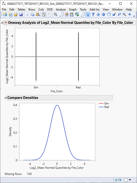
We can see from the plots above that the sample means and densities now overlap and display a normal distribution. The normalized data are used in subsequent analyses. The next step is to separate the sample data and restructure the table into a wide![]() A data table in which variables are columns and samples are rows. format.
A data table in which variables are columns and samples are rows. format.
Reformatting the Data Table
Splitting the Table
The first step in formatting the table is to split the data from the two samples into separate columns using the Split command.
| 8 | Select Tables > Split to open the Split platform. |
| 8 | Specify File_Color as the Split By column. |
| 8 | Specify new Log2_Mean Normal Quantiles by File_Color as the Split Column. |
| 8 | Specify Illumina_ID and File_Root as the Groups. |
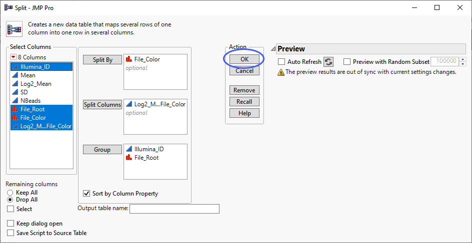
| 8 | Click . |
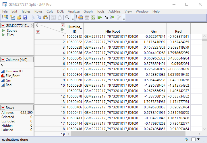
The GSM2277217_Split.jmp table places the data from the red and green samples side by side for each probe set. The table contains 622399 rows, exactly half of the 1,244,798 rows of the original stacked table. Unneeded columns in the original table have been discarded. This is still a tall table.
Converting the table from tall format to wide format.
The tall table must be converted to wide format for analysis.
| 8 | Select the two data columns. |
| 8 | Right-click on the column headings and select New Formula Column > Combine > Difference. |
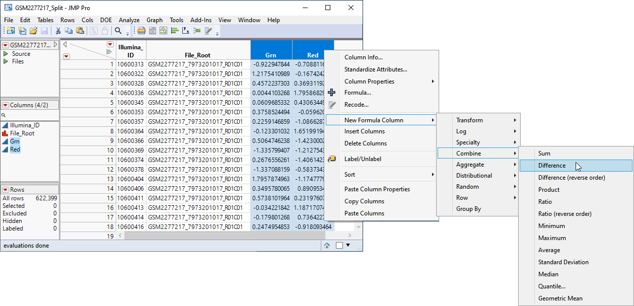
This adds a new column (highlighted below) to the table containing the log2-based logit of beta, the ratio of methylated to unmethlyated signal.

Split the table again.
| 8 | Select Tables > Split to open the Split platform. |
| 8 | Specify Illumina_ID as the Split By column. |
| 8 | Specify new Grn-Red as the Split Column. |
| 8 | Specify File_Root as the Group. |
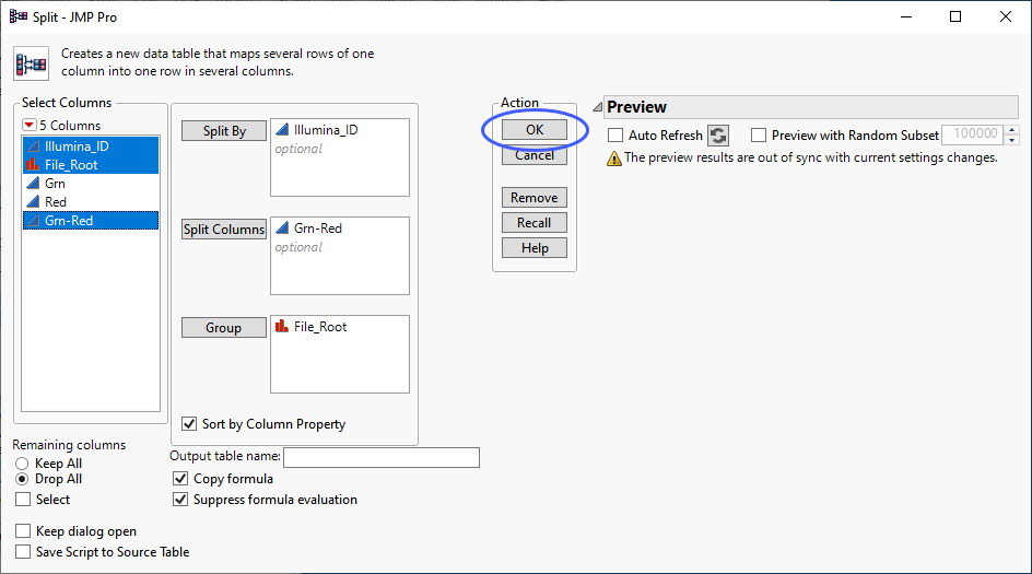
| 8 | Click . |
The following table is generated.
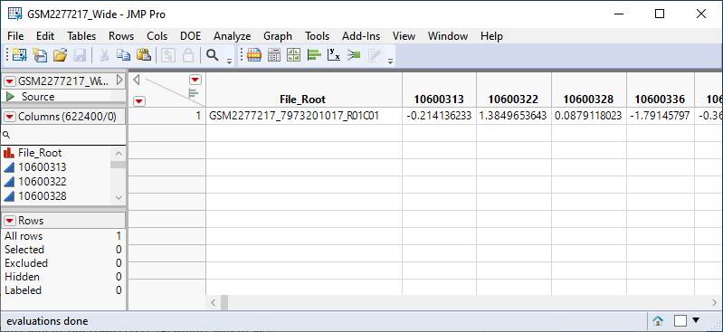
The GSM2277217_Wide table has been converted to wide format and is ready for analysis. It has 622400 columns and one row.
Note: The number of rows in the final table of this import procedure will always equal the number of green rows = red rows divided by two.