Importing MTX Files

Single cell RNA-seq methodology enables researchers to assess the expression profiles of individual cells within a mixed population. Generating these profiles is a destructive process, so each profile represents a static snapshot of a cell at a specific point along a developmental progression. However, by taking samples at different times, researchers can assemble a reasonably complete understanding of cells' progression through development.

Data from single-cell RNA-seq experiments are often stored as a sparse matrix with genes in rows and each cell comprising a column (Tall format A data table in which variables in rows and samples are in the columns). This format system consists of exactly three files: one with suffix .mtx, and the other two with some type of text format (usually with suffix .tsv, but can be either .csv or .txt). The files used in this example contain data from an experiment in which sequencing of bronchoalveolar lavage fluid (BALF) of mine workers with silicosis and their co-workers who did not develop silicosis and were downloaded from GEO. A zip file containing these files is available here for you to download.

•

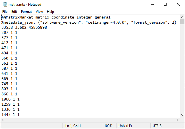
The .mtx file must contain data with three columns corresponding to row index, column index, and value (counts). Initial lines beginning with % are ignored, as is the first data line, which typically contains the dimensions of the sparse matrix and number of nonzero entries. The example shown below shows the matrix.mtx file has two rows containing general information. The data starts on line three with 3 columns of data per line. The first data line shows the size of the matrix (in this example, 33538 rows, 33602 columns, and 45855898 non-zero values). The next row shows that in column 207, the value in column 1 is 1.

•

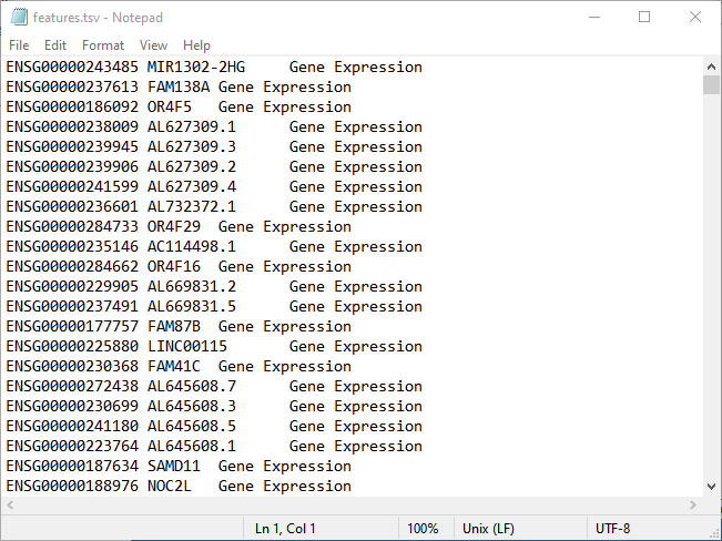
One of the text files must have one of the following substrings in its name: row, gene, or feature. This file contains the row labels of the sparse matrix, representing the names of all the genes in the study. It can also contain gene-wise information, such as gene length, chromosomal position, etc. This file must be sorted correctly to match the row indices in the .mtx file. If it only has one column, then it is assumed to be headerless, with data beginning on the first line. If it has more than one column, it may or may not have a header. If no header is present, data begins on the first line. If a header is present, it is assumed to be on the first line and data begins on the second line. The example below shows the features.tsv file has no header. The data starts on line 1 with three columns per line.

•

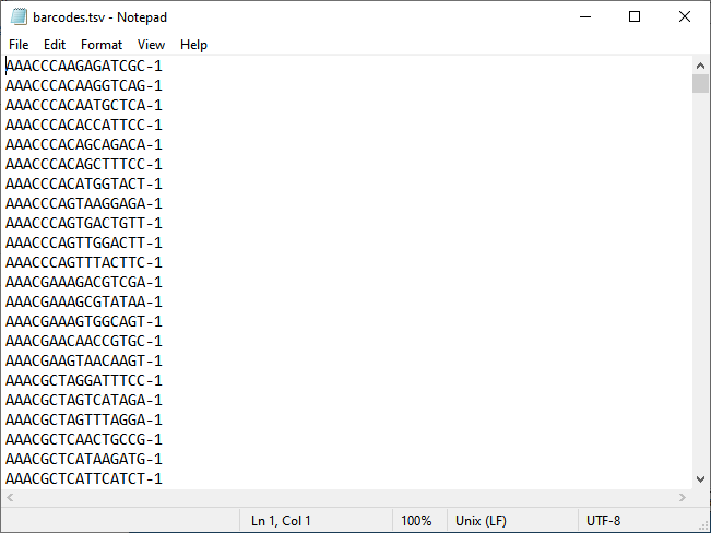
The other text file must have one of the following substrings in its name: col, barcode, cell. This file contains column label of the sparse matrixes, representing the cells in the study, and must be sorted correctly to match the column indices in the .mtx file. If it only has one column, then it is assumed to be headerless, with data beginning on the first line. If it has more than one column, then headers are assumed to be on the first line and data begins on the second line. The example below shows the barcodes.tsv file has one column.

Note: These files must be saved to the same folder, preferably without any other files.

Importing the Files into JMP PRO

In this example, we import the files shown above.

Select File > Import Multiple Files.... A Multiple File Import window opens.

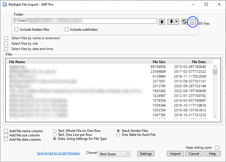
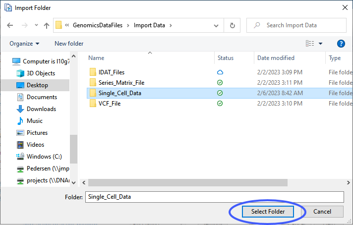
Click to open an Import Folder window. Navigate to the folder containing the files to be imported and click .

The Multiple File Import window shows the files to be imported.

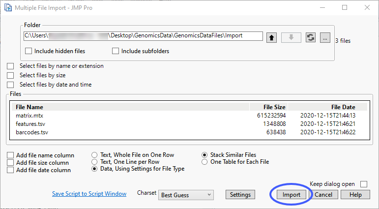
Click to import the files.

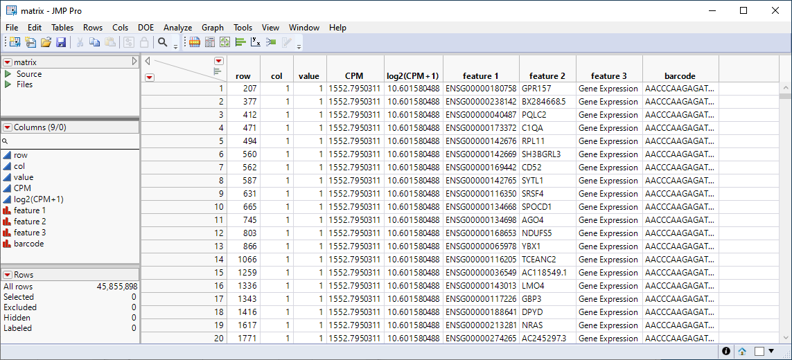
The output contains four files: the original three files with additional columns added, and a fourth wide table created by splitting the mtx table, effectively converting the data from a sparse to a dense format.

The mtx file output contains the following columns: row, col, value, CPM, log₂(1+CPM), and columns (Gene_ID, Ensemble_ID, and barcode) joined from the two text files. CPM is counts per million, computed by dividing each value by its column sum and multiplying by 1e⁶. This table is still a sparse matrix, containing only those cells with a nonzero value.

The wide table A data table in which variables are columns and samples are rows. contains values from the log₂(1+CPM) column and 0s elsewhere. Its column names are created from the first column in the row text file, in other words genes become the columns and barcodes (cell IDs) the rows, the transpose of the original sparse matrix.

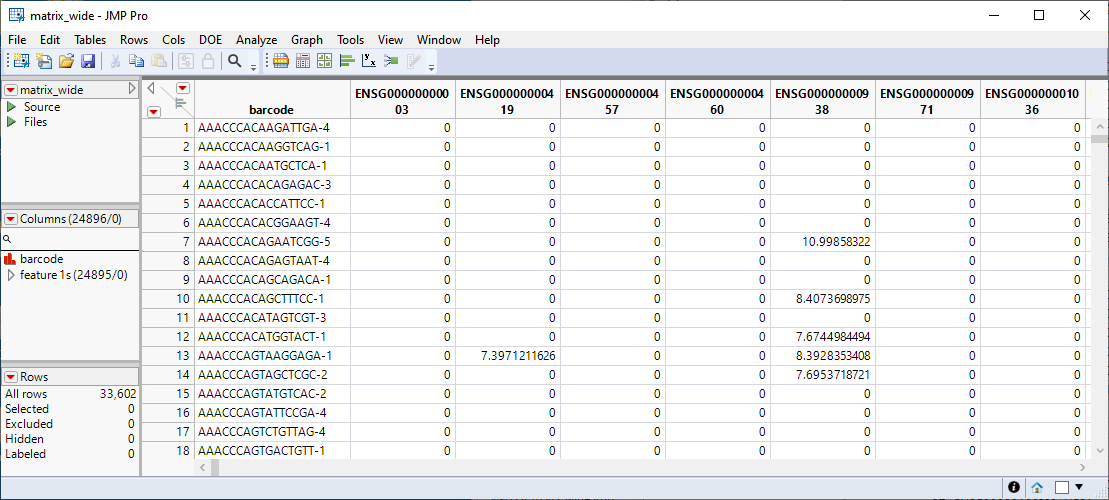
The matrix_wide.jmp table shown above is a dense table with all cells included. Most of the cells contain zeros, indicating no counts were registered. Nonzero values represent the log₂(1+CPM) transform of the original data. This transform should generally be appropriate for single-cell RNA sequencing count data1.

If some other transform or the original count data is desired in a wide table, use the following steps:

In the mtx output table, create the desired data in a column.

Click Tables > Split, specify the new data column in Split Columns, the desired column name column in Split By, and other columns in other fields as desired. Click .

(Optional) Select all of the wide data columns, Right-Click > Group Columns. Double click the group name and change it to a meaningful name. Select the columns and click Cols > Utilities > Compress Selected Columns. Click the table red triangle near the upper left corner and select Compress File When Saved.

Select all of the wide data columns. Right-Click > Standardize Attributes > Recode. Change missing value to 0 and click .

Save the table.

The tables that you have imported should be ready for analysis.