Note
: JMP Clinical uses a special protocol for data including non-unique Findings test names. Refer to
How does JMP Clinical handle non-unique Findings test names?
for more information.
Note
: Refer to
Distribution Reports
for a description of the general analysis performed by the JMP Clinical distribution reports.
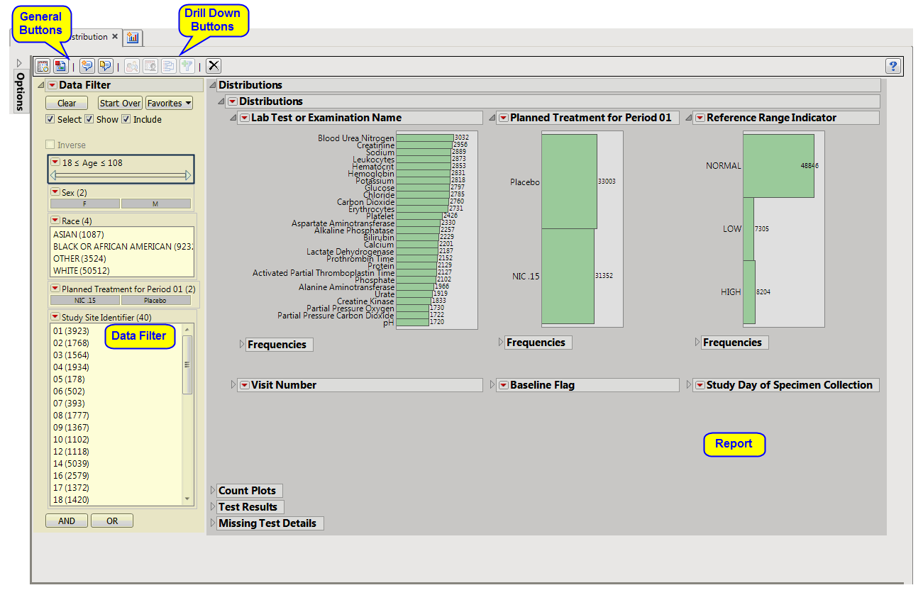
Running
Findings Distribution
for
Nicardipine
using default settings generates the
Report
shown below.
The
Report
contains the following sections:
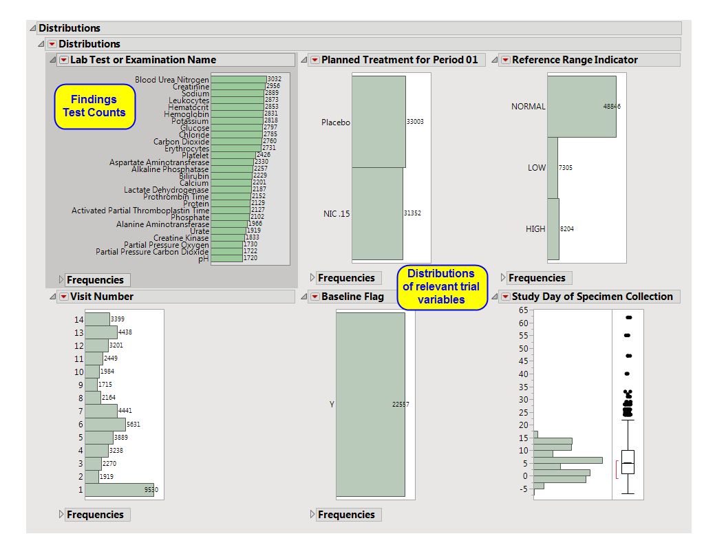
Contains
Histogram
s
to display the
distribution
of Findings tests taken during the study and other relevant
variables
for the selected Findings domain.
|
•
|
One Findings Test
Counts Graph
.
|
This graph shows a
Histogram
displaying how often measurements were taken for each findings test (
xxTESTCD
) during the study.
|
•
|
A set of
Distributions
.
|
These display counts and histograms of relevant
variables
in the Findings data set. A
distribution
of subjects on the
Actual
,
Planned
, or
Specified Treatment
is shown as well as other findings variables (if present). Findings variables displayed can include the Findings
Body System
(
xxBODSYS
),
Reference Range Indicator
(
xxNRIND
), the
Category for the Test
(
xxCAT
) and
Subcategory
(
xxSCAT
), the
Categorical Findings Result
(
xxSTRESC
, only displayed for categorical findings domains), the
Visit
and
Time Points
at which findings were taken (
VISIT
and
xxTPT
),
Baseline Flag
(
xxBLFL
), and the
Study Day
.
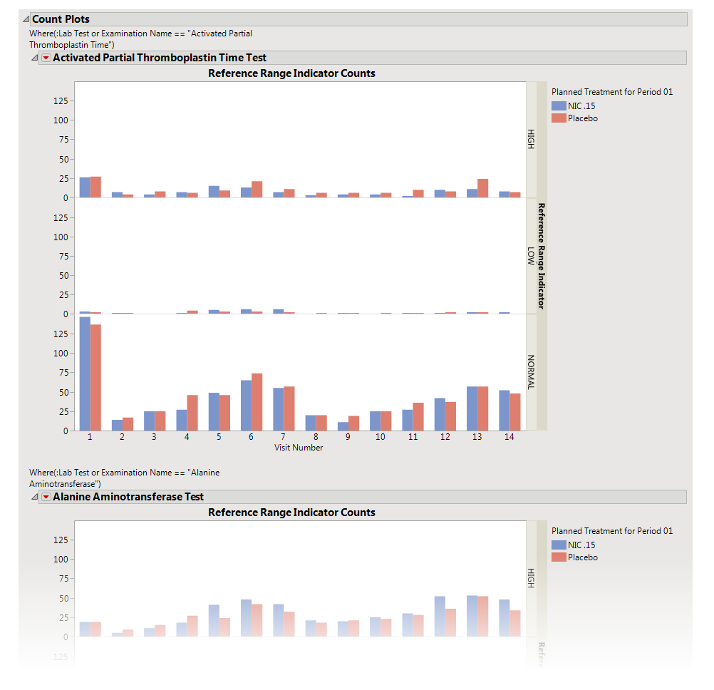
The
Count Plots
section is shown below. This section is shown only when the
xxNRIND
variable
and either
VISIT
or
VISITNUM
is found in the Findings data set.
|
•
|
These plots show the
distribution
of measurements across categories of the
Reference Range Indicator
variable (
xxNRIND
). For example, you can see how many laboratory measurements for a given test were categorized as
HIGH
,
NORMAL
, or
LOW
based on values of the
Reference Range Upper Limit
and
Reference Range Lower Limit
(
LBSTNRLO
and
LBSTNRHI
, respectively). The graph contains bars representing the counts within each category for each treatment across
Study Visits
(
VISIT
or
VISITNUM
).
Contains One-way Analyses (
ANOVA
) for each test that has numeric measurement results (
xxSTRESN
values), Contingency Analyses for each Findings test that has character results (
xxSTRESC
values but missing
xxSTRESN
values), or both.
Note
: This section can display analyses for numeric and/or categorical findings tests, depending on the tests found within the chosen analysis Findings domain.

It contains
one or both
of the following elements:
|
•
|
A set of
Oneway Analyses for Numeric Findings Tests
.
|
Each analysis represents an Analysis of Variance (
ANOVA
) for each numeric Findings test (tests that contain
nonmissing
values for
xxSTRESN
) to compare measurements taken across different treatment
arms
. You can click the
Oneway ANOVA
outline box below each plot to show the statistical results of the analysis.
Note that this analysis is across
all
measurements taken during the study and should be used to get an idea of possibly significant differences in measurements across treatment arms. This is a simple
model
. You can fit a more appropriate model that accounts for the repeated measures taken for subjects, as well as initial baseline measurements, with the
Findings ANOVA
report.
See the JMP
Fit Y by X
platform for more details about Oneway Analysis.
|
•
|
A set of
Contingency Analyses for Categorical Findings Tests
.
|
Each analysis represents a contingency analysis for each categorical test (tests that contain
nonmissing
values for
xxSTRESC
but are
missing
values for
xxSTRESN
) to compare measurements taken across different treatment arms. A
Mosaic Plot
shows the proportion of measurements for values of
xxSTRESC
across treatment arms. You can click the
Tests
outline box below each plot to display tests for significant differences in the proportion of values across treatment.
See the JMP
Fit Y by X
platform for more details about Contingency Analysis.
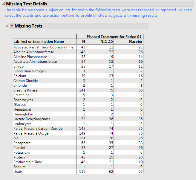
Contains tables displaying subject counts for tests that were either not recorded, or that were recorded but have missing measurement values (of
xxSTRESN
and/or
xxSTRESC
).
Note
: This section is
not
shown if all subjects have
nonmissing
measurements taken for all Findings tests recorded.
|
•
|
A
Missing Tests
Table.
|
This table displays subject counts for which Findings tests were either not reported or not recorded. For example, the number of subjects that did not have any record taken for the
ALT
lab test in the
LB
domain is displayed in this table for the
ALT
test row.
|
•
|
A
Missing Tests Results
Table.
|
This table displays subject counts for any Findings test was that was recorded, but has a missing measurement value (missing an
xxSTRESN
value for numeric tests or missing an
xxSTRESC
for categorical tests). This table differs from the
Missing Tests
Table in that a record was reported for the test for that subject, but the
measurement value
was missing.
This enables you to subset subjects based on demographic characteristics and study site. Refer to
Data Filter
for more information.
|
•
|
Profile Subjects
: Select subjects and click
|
|
•
|
Show Subjects
: Select subjects and click
|
|
•
|
Cluster Subjects
: Select subjects and click
|
|
•
|
Demographic Counts
: Select subjects and click
|
|
•
|
Click
|
|
•
|
Click
|
|
•
|
Click
|
|
•
|
Click
|
|
•
|
Click the
arrow to reopen the completed report dialog used to generate this output.
|
|
•
|
Click the gray border to the left of the
Options
tab to open a dynamic report navigator that lists all of the reports in the review. Refer to
Report Navigator
for more information.
|

Additional Filter to Include Subjects
2
,
Merge supplemental domain
,
Include the following findings records:
,
Additional Filter to Include Findings Tests
,
Select the population to include in the analysis
,
By Variables
Subject-specific filters must be created using the
Create Subject Filter
report prior to your analysis.
For more information about how to specify a filter using this option, see
The SAS WHERE Expression
.