This analysis visualizes peak values for lab measurements pertaining to
Hy’s Law
for detecting potential liver toxicity for all subjects across treatment
arms
. Lab measurements for Bilirubin (BILI), Alanine Aminotransferase (
ALT
), Aspartate Aminotransferase (AST), and Alkaline Phosphatase (ALP) are divided by the upper limit of normal (ULN) and displayed in a
scatterplot
matrix annotated with Hy's Law reference lines (2*ULN of BILI, 3*ULN of ALT).
This analysis also creates reports of the
distributions
of relevant liver test
variables
, tables of missing tests and categorized liver elevation levels, and displays of the peak liver test values by Study day.
Note
: This analysis can still be run on a blinded study but certain components of the reports are suppressed.
Note
: JMP Clinical uses a special protocol for data including non-unique Findings test names. Refer to
How does JMP Clinical handle non-unique Findings test names?
for more information.
Running this report with the
Nicardipine
sample setting generates the report shown below.
The
Report
contains the following elements:
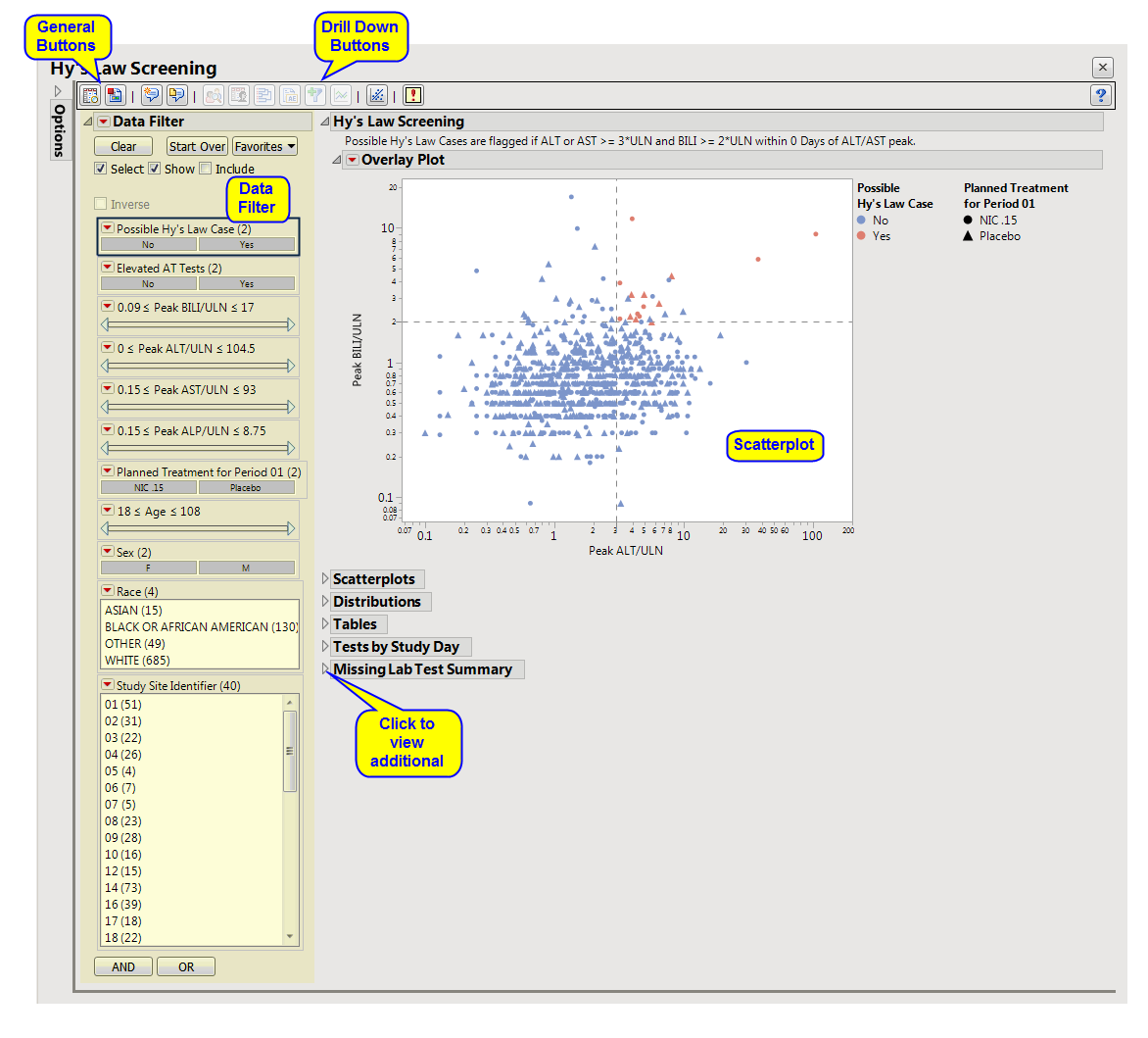
Displays an overall
scatterplot
of peak
ALT
,
AST
,
BILI
, and
ALP
measurements across the study, with color used to flag subjects meeting Hy's Law criteria.
The
Hy’s Law Screening
section consists of the following elements:
|
•
|
One
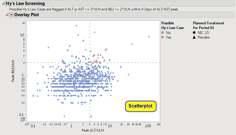
Overlay Plot
of Hy's Law Lab Tests.
|
This plot shows maximum laboratory values for the Alanine Aminotransferase (
ALT
), Aspartate Aminotransferase (
AST
), Total Bilirubin (
BILI
), and Alkaline Phosphatase (
ALP
) laboratory tests. The values are log
2
transformed (this can be changed to log
10
or
no transformation
in the report
dialog
) and normalized by the Upper Limit of Normal (
LBSTNRHI
). Reference lines are drawn by default at 3*
ULN
for
ALT
and
AST
and 2*
ULN
for
BILI
and
ALP
. These reference limits can be customized on the dialog.
These limits are also used to create the Hy's Law indicator flag. Subjects with a test value exceeding 3*
ULN
for
ALT
or
AST
(signs of hepatocellular injury) accompanied or followed by elevation of 2*
ULN
or greater for the
BILI
test have a "Yes" value for the
Hy's Law Case
variable
created. A note defining the Hy's Law flag is located
above
the
scatterplot
matrix. For example, with the default settings the note is as follows: "
Hys Law Cases are flagged if ALT or AST >= 3*ULN and BILI >= 2*ULN within 0 Days of ALT/AST peak.
" You can change the number of days following
ALT
/
AST
elevation for which to look for BILI elevation to flag possible Hy's Law cases on the report dialog. Subjects in the plot are colored by the Hy's Law criteria (
red
for "Yes",
blue
for "No") and marked by their treatment
arm
. You can choose to label the quadrants of Hy's Law (Cholestasis, Hy's Law, and Temple's Corollary) in the
bottom left
scatterplot through a check box option on the dialog.
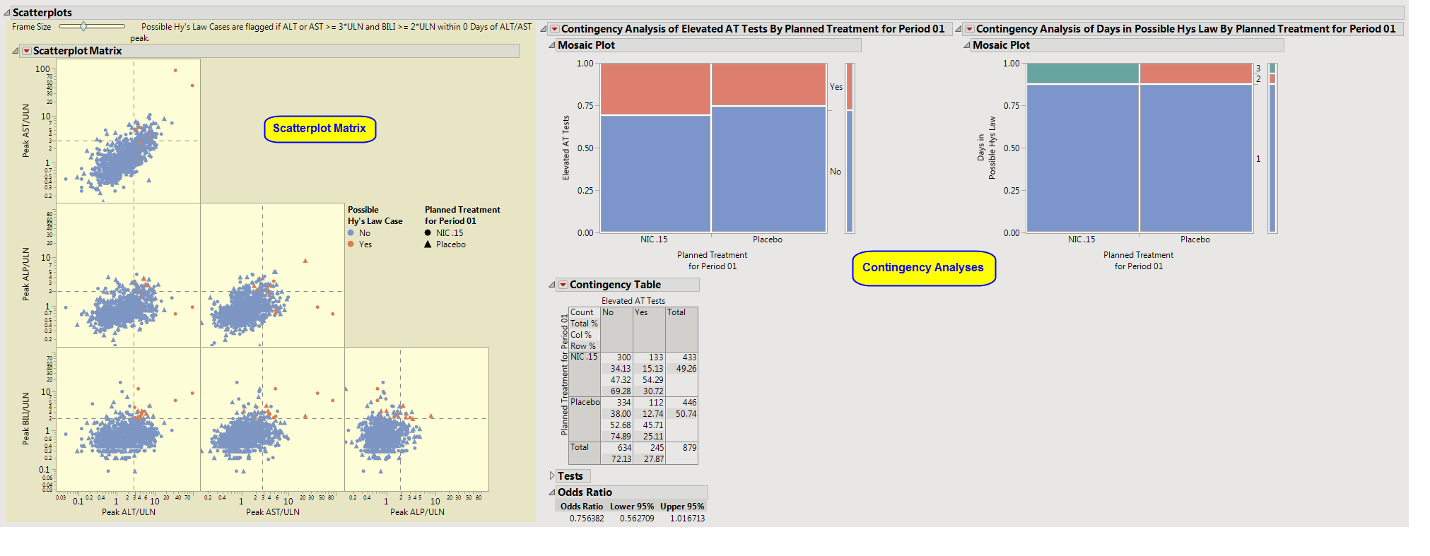
Displays scatterplots of peak
ALT
,
AST
,
BILI
, and
ALP
measurements across the study, with color used to flag subjects meeting Hy's Law criteria. Two contingency analyses show duration of Hy's Law and incidence of
ALT
or
AST
elevation by treatment.
The
Scatterplots
section contains the following elements:
|
•
|
One
Scatterplot Matrix
of Hy's Law Lab Tests.
|
Tip
: Adjust the size of the
scatterplot
matrix using the
Frame Size
slider, located at the
upper left
corner of the tab.
This plot shows maximum laboratory values for the Alanine Aminotransferase (
ALT
), Aspartate Aminotransferase (
AST
), Total Bilirubin (
BILI
), and Alkaline Phosphatase (
ALP
) laboratory tests. The values are log
2
transformed (this can be changed to log
10
or
no transformation
in the report
dialog
) and normalized by the Upper Limit of Normal (
LBSTNRHI
). Reference lines are drawn by default at 3*
ULN
for
ALT
and
AST
and 2*
ULN
for
BILI
and
ALP
. These reference limits can be customized on the dialog.
These limits are also used to create the Hy's Law indicator flag. Subjects with a test value exceeding 3*
ULN
for
ALT
or
AST
(signs of hepatocellular injury) accompanied or followed by elevation of 2*
ULN
or greater for the
BILI
test will have a "Yes" value for the
Hy's Law Case
variable
created. A note defining the Hy's Law flag is located
above
the scatterplot matrix. For example, with the default settings the note is as follows: "
Hys Law Cases are flagged if ALT or AST >= 3*ULN and BILI >= 2*ULN within 0 Days of ALT/AST peak.
" You can change the number of days following
ALT
/
AST
elevation for which to look for BILI elevation to flag possible Hy's Law cases on the report dialog. Subjects in the plot are colored by the Hy's Law criteria (
red
for "Yes",
blue
for "No") and marked by their treatment arm. You can choose to label the quadrants of Hy's Law (Cholestasis, Hy's Law, and Temple's Corollary) in the
bottom left
scatterplot through a check box option on the dialog.
|
•
|
Two
Contingency Analyses
.
|
Two contingency analyses are shown in addition to the scatterplot matrix if any subjects were flagged as Hy's Law or if subjects experienced elevated
ALT
/
AST
tests. The first contingency analysis shows a
Mosaic Plot
and count matrix (
Contingency Table
) of how many days subjects were experiencing lab test elevations that met the Hy's Law flag across treatment arms. This plot and analysis can give valuable insight into the severity and duration of lab test elevation that could signify liver injury. The second contingency analysis compares the incidence of subjects who experience hepatocellular injury (
ALT
/
AST
elevation >= 3*
ULN
or as defined by dialog option) across treatment
arm
. A statistical test is provided along with counts that can signify if there is a statistically significant higher number of subjects experiencing liver injury while on the drug versus the placebo. This can give insight into possible drug induced liver injury issues.
The
Scatterplot Matrix
and the
Mosaic Plot
s
in the
Contingency Analyses
are interactive and linked. You can select subjects in the scatterplot or in the colored boxes of the
mosaic plot
to see where they lie in the analysis. For example, it might be useful to select the boxes in the mosaic plot for the
Days in Hy's Law
contingency analysis for the treatment group to see the max lab values for those subjects in the scatterplots. In addition, you can select the points using the values of the
Hy's Law Case
and
Treatment
legend on the scatterplot. Once subjects are selected, you can choose from any of the
Action Button
-downs (
and
are highly informative to look at the subjects' entire safety profiles) to further explore possibly liver injury safety issues in the trial.
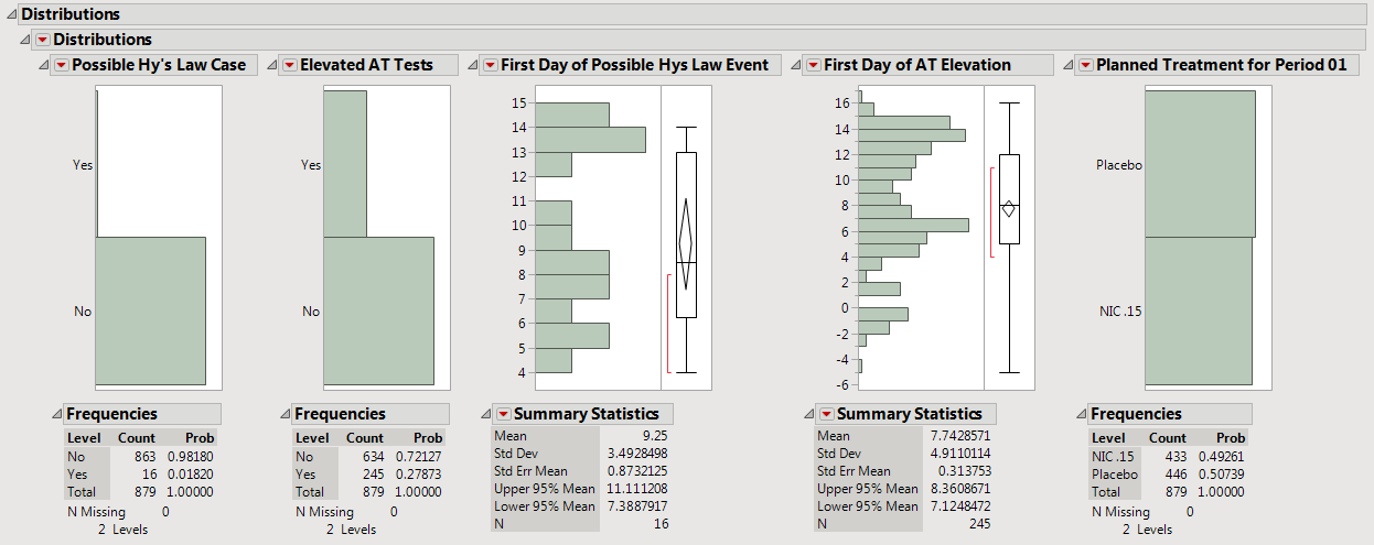
The
Distributions
section is shown above and contains the following elements:
|
•
|
A set of
Distributions
.
|
These display histograms and summary statistics of
variables
from the Findings data set that are relevant to a
Hy’s Law
analysis.
Distributions
of subjects on the
Actual
,
Planned
, or
Specified Treatment
(grouped by age, sex, race, and other factors) are displayed.
Contains tables corresponding to AT Test Elevation and Potential
Hy’s Law
Cases, as well as counts and percentages for elevation categories for each liver test.

|
•
|
One
AT Test Elevation and Potential Hy’s Law Cases
table.
|
Note
: This table is shown only if at least one subject has a value of “
Yes
” for
Elevated AT Tests
.
This table lists subject count and percentages by treatment
variable
for subjects experiencing
ALT
or
AST
Elevation, or those defined as a
Hy’s Law
Case, or both.
|
•
|
A table of
Counts and Percents
for elevation categories for each liver test.
|
All tables are associated with the
Local Data Filter
(located on the
right
side). You can use this filter to subset the tables based on variable filters. You can select cells of these tables (either counts or percents) to select the corresponding rows in the data table.
Missing Test Result
is calculated as count (and percent) of subjects who had no record of a specific test (there is no row in the
lb
data set for the respective
LBTEST
for the subject) at any day of the study, have no nonmissing measurement(s) for the recorded test (
LBSTRESN
is a
missing value
), or are missing the upper limit of normal reference limit (
LBSTNRHI
is a missing value).
Important
: The counts and percentages for
Missing Test Result
on this section are calculated out of all subjects that have at least one nonmissing result for at least one of the liver lab tests. The counts shown on the
Missing Lab Test Summary
section include subjects that had no record or were missing all values for all four liver lab tests.
Note
: These tables are derived from the same data table that the
Hy’s Law Screening
,
Scatterplots
, and
Distributions
sections are derived from, so any selections that you make are reflected across those tabs.
|
•
|
One
Local Data Filter
.
|
|
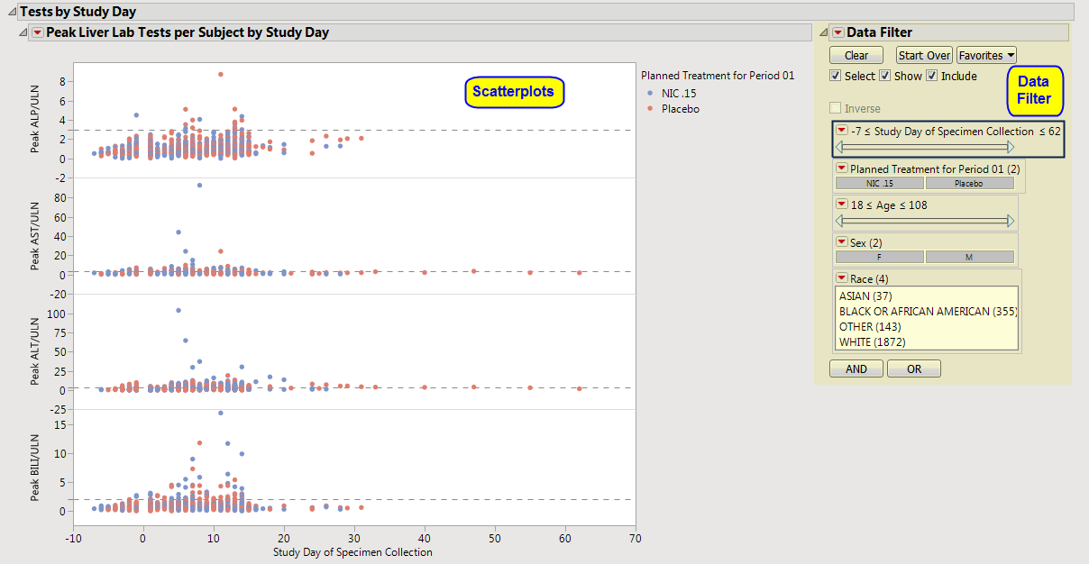
•
|
For each of the four liver tests, peak values are shown on the
Y
axis for each subject, for each
Study Day
(
LBDY
on the
X
axis).
Points
are colored by treatment group.
Reference lines
are drawn according to typical reference limits (or those custom reference lines specified on the report
dialog
).
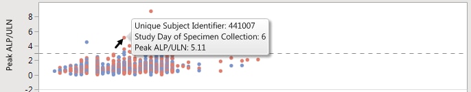
You can select points in the graph and their corresponding rows in the data table become selected. Click
to see the data table reflecting any selections that you have made.
|
•
|
One
Data Filter
.
|
Use the data filter to subset the
scatterplot
matrix and associated data table by any of the available criteria. For example, you could filter the data by females between 40 and 50 years old. Drag the
Age
slider ends, or type over minimum and maximum age values to obtain an exact age range. The number of matching rows, selected graph points, and data table selections are updated accordingly.
Contains a table showing counts of subjects for which the relevant Hy's Law lab tests were
not
measured.

The
Missing Lab Test Summary
section contains the following elements:
|
•
|
One table of
Counts of Subjects Missing Liver Lab Records
.
|
This table lists counts of subjects across treatment
arms
for which the relevant liver tests were not performed or measured. It is common in clinical trials to measure these laboratory tests in order to monitor for potential liver injury.
Important
: The counts shown on this section include subjects that had no record or were missing all values for all four liver lab tests. The counts and percentages for
Missing Test Result
on the
Tables
section are calculated out of all subjects that have at least one nonmissing result for at least one of the liver lab tests.
The counts in the table columns are
interactive
. You can select the numbers to select the corresponding subjects for which a test was not measured. You can then use the
Down Buttons
to show those subjects or profile them for further analysis.
This enables you to subset your data based on demographics, test results, and/or study site. Refer to
Data Filter
for more information about how to use the
Data Filter
.
|
•
|
Profile Subjects
: Select subjects and click
|
|
•
|
Show Subjects
: Select subjects and click
|
|
•
|
Cluster Subjects
: Select subjects and click
|
|
•
|
Demographic Counts
: Select subjects and click
|
|
•
|
Graph Time Profiles
: Select subjects and click
|
|
•
|
Liver Lab Shift Plots
: Click
|
|
•
|
Click
|
|
•
|
Click
|
|
•
|
Click
|
|
•
|
Click
|
|
•
|
Click the
arrow to reopen the completed report dialog used to generate this output.
|
|
•
|
Click the gray border to the left of the
Options
tab to open a dynamic report navigator that lists all of the reports in the review. Refer to
Report Navigator
for more information.
|

This report requires lab results for bilirubin, alanine aminotransferase, aspartate aminotransferase, and alkaline phosphatase. At least one of the standardized short name character strings listed in the following table must be present in the
LBTESTCD
column for each lab result.
|
Lab Test
1
:
|
|
|
Note
: If neither
BILI
nor
TBIL
are found, the report searches for and uses
TBILI
,
TBL
,
BILT
,
BILTOT
, and
BIL
(in that order).
|
|
|
Note
: If neither
ALP
nor
ALKP
are found, the report searches for and uses
ALK
and
APH
, in that order.
|
Note
: You can specify the correct tests on the
Tests
tab of the
dialog
if the relevant tests are not coded using the common strings listed here,
Time Lag (in Days) for Classifying Hy’s Law Cases
,
Normalize laboratory values by:
,
Calculate baseline as:
Additional Filter to Include Subjects
2
,
Merge supplemental domain
,
Select the population to include in the analysis
,
By Variables
Lab Test Short Name for Bilirubin
,
Lab Test Short Name for Alanine Aminotransferase
,
Lab Test Short Name for Aspartate Aminotransferase
,
Lab Test Short Name for Alkaline Phosphatase
Create Hy’s Law 3D Plot
,
Use log scaling to display findings test measurements
,
Label Hy’s Law quadrants
,
Set custom reference lines for Hy’s Law plots
,
Set reference line for bilirubin
,
Set reference line for transaminase tests
Subject-specific filters must be created using the
Create Subject Filter
report prior to your analysis.
For more information about how to specify a filter using this option, see
The SAS WHERE Expression
.