This report calculates
Mahalanobis distance
based on available data, using the equation
 , to identify subject inliers and outliers in multivariate space from the multivariate
mean
. Refer to the JMP documentation on
Mahalanobis Distance Measures
for statistical details. It also generates results by site to see which sites are extreme in this multivariate space.
, to identify subject inliers and outliers in multivariate space from the multivariate
mean
. Refer to the JMP documentation on
Mahalanobis Distance Measures
for statistical details. It also generates results by site to see which sites are extreme in this multivariate space.
Mahalanobis distance is plotted on the log scale to allow for easier examination of small scores. The reference line is derived from a
transformation
of the mean of the approximate
chi-square
distribution
.
This report attempts to use as much data as possible. Along with sex and age, it takes all findings test codes by visit number and time number (if available), as well as frequencies of all event and intervention codes per subject. Of course, doing so can lead to missing data particularly for studies that do not appear to have a fixed number of visits or with lots of dropouts. Because Mahalanobis distance cannot be calculated with lots of missing data present, there is an option to delete
variables
with at least
X
% of missing data
1
based on the selected
population
and filters (default of 5%). Of remaining variables, scores are computed for those subjects with complete data. The general strategy of this report is to use as many variables as possible, while letting a few early dropouts fall out of the analysis.
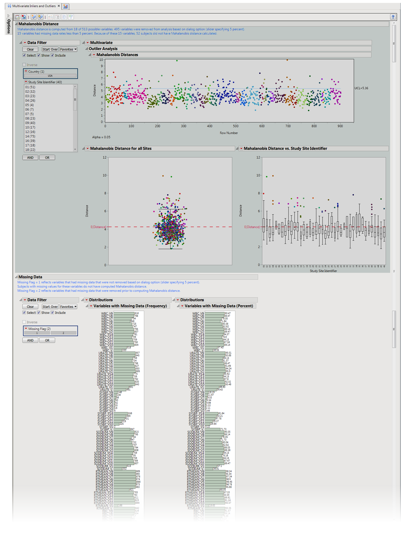
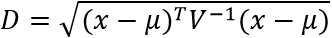
Presents plots of
Mahalanobis distance
of all subjects (distance is from the multivariate
mean
), colored by study site, and
Box Plot
s presented by sites.
|
•
|
One JMP
Mahalanobis Distances
plot to identify significant outliers. In the
Mahalanobis Distances
plot shown above, the distance of each specific
observation
(row number) from the
mean
center of the other observations of each row number is plotted. Those outlier points residing above the dotted line correspond to those rows that warrant the most attention due to their significant distance from the mean center of all other observations.
|
The first
box plot
shows all subjects for which Mahalanobis Distance is calculated. Values closer to
zero
(0) reflect subjects that are close to the multivariate mean of the
variables
(inliers). Larger values represent subjects that are extreme in multivariate space. The
square
of Mahalanobis Distance is distributed as
chi-square
with
k
degrees of freedom, where
k
is the number of variables used in the calculation of Mahalanobis Distance. The redline reflects the
square root
of
k
. The second figure shows box plots by study site. This allows the analyst to determine how different sites are from the multivariate mean.
|
•
|
One
Data Filter
.
|
Enables you to subset subjects based on country of origin and study site. Refer to
Data Filter
for more information.
Details
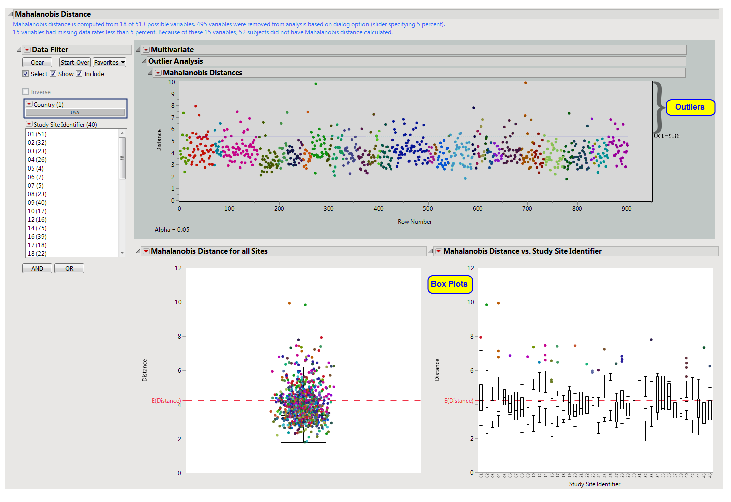
variables
that contain missing data that prevented
Mahalanobis distance
from being calculated for certain subjects (
Flag = 1
) or variables that were dropped from analysis based on the
dialog
option
Remove variables from analysis with a missing data percentage of at least:
. By default, variables with
5
% or more of missing data are
not
used in the calculation of Mahalanobis Distance. Data are presented either as counts (
left
) or percentages (
right
) reflect the number of values that are missing for each variable. Opening the data table shows the percentage of missing data for each test.
|
•
|
One
Data Filter
.
|
Enables you to subset histograms based on date characteristics. Additional terms can be added from the data table using the
and
buttons of the filter.
|
•
|
Profile Subjects
: Select subjects and click
|
|
•
|
Show Subjects
: Select subjects and click
|
|
•
|
Cluster Subjects
: Select subjects and click
|
|
•
|
Demographic Counts
: Select subjects and click
|
Output includes one summary data set (named
csass_sum_XXX
2
, by default) containing one record per subject with pre-dosing data, one data set of all pairwise distances within the
covariate
subgroups (named
csass_alldist_XXX
, by default), one data set containing minimum pairwise distances for each covariate subgroup (named
csass_mindist_XXX
), by default), one data set per covariate subgroup containing pairwise distances (named
csass_p_Y_XXX
, by default, where
Y
is indexed 1 to the number of covariate subgroups) and one data set per covariate subgroup containing the
distance matrix
of subjects within the covariate subgroup (named
csass_Y_XXX
, by default, where
Y
is indexed 1 to the number of covariate subgroups).
Variable names for Findings data are concatenated with the abbreviation of the Findings test and the visit number (
V
). For example,
DIABP_V2
is the diastolic blood pressure at visit 2. If there are multiple measurements at Visit 2, then it is the average. If there are multiple time points on a single visit, a time number is appended. For example,
DIABP_V2_T1
would be the diastolic blood pressure at time point 1 at visit 2 (or the average, if multiple measurements are taken);
DIABP_V2_T2
would be the diastolic blood pressure at time point 2 at visit 2.
|
•
|
Click
|
|
•
|
Click
|
|
•
|
Click
|
|
•
|
Click the
arrow to reopen the completed report dialog used to generate this output.
|
|
•
|
Click the gray border to the left of the
Options
tab to open a dynamic report navigator that lists all of the reports in the review. Refer to
Report Navigator
for more information.
|
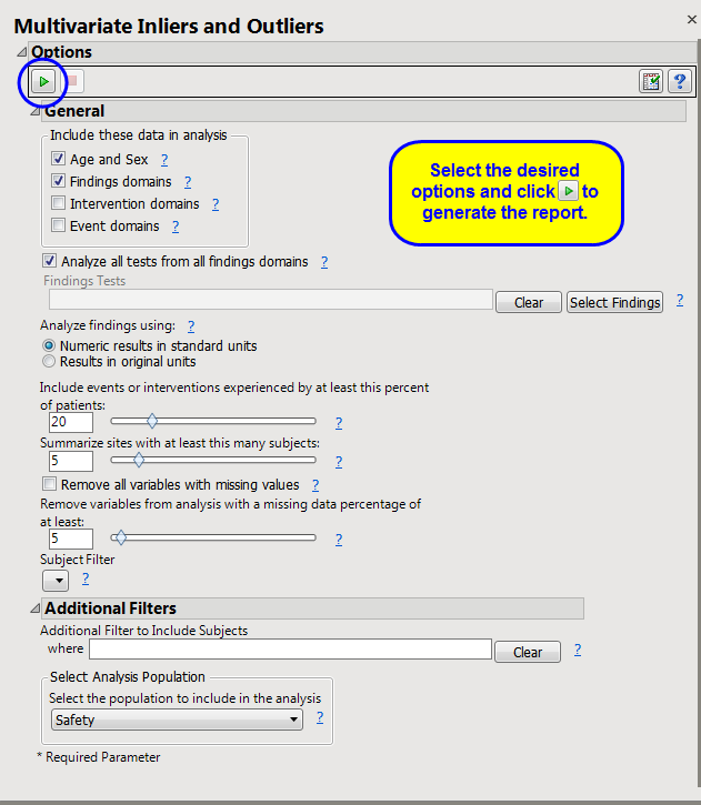
Analyze all tests from all findings domains
,
Findings Tests
,
Analyze findings using:
,
Include events or interventions experienced by at least this percent of patients:
,
Summarize sites with at least this many subjects:
,
Remove all variables with missing values
,
Remove variables from analysis with a missing data percentage of at least:
The
_XXX
designation is used to designate a one- to three-digit number that is added sequentially to prevent overwriting of existing data sets.
Subject-specific filters must be created using the
Create Subject Filter
report prior to your analysis.
For more information about how to specify a filter using this option, see
The SAS WHERE Expression
.