The AE Severity ANOVA report screens all adverse events by performing a mixed-model analysis of variance, with average ranked severity score as the dependent variable and customizable fixed and random effects. A separate ANOVA is fit for each distinct adverse event. Volcano plots and other output enable efficient screening of adverse event severities that differ between treatment groups. If a patient has multiple instances of a particular adverse event, then those scores are averaged to form a single score for analysis.
Running this report for Nicardipine using default settings generates the report shown below.

The Results contains the following elements:
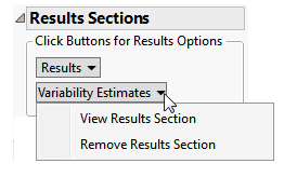
This pane enables you to access and view the output plots and associated data sets on each tab. Use the drop-down menu to view the section in the Results pane or remove the section and its contents from the Results pane.
This section shows the primary results from the analysis, including Volcano Plots and various analyses on least squares means.
The Results section is similar to the LB Results section except that adverse events, rather than findings, are plotted.
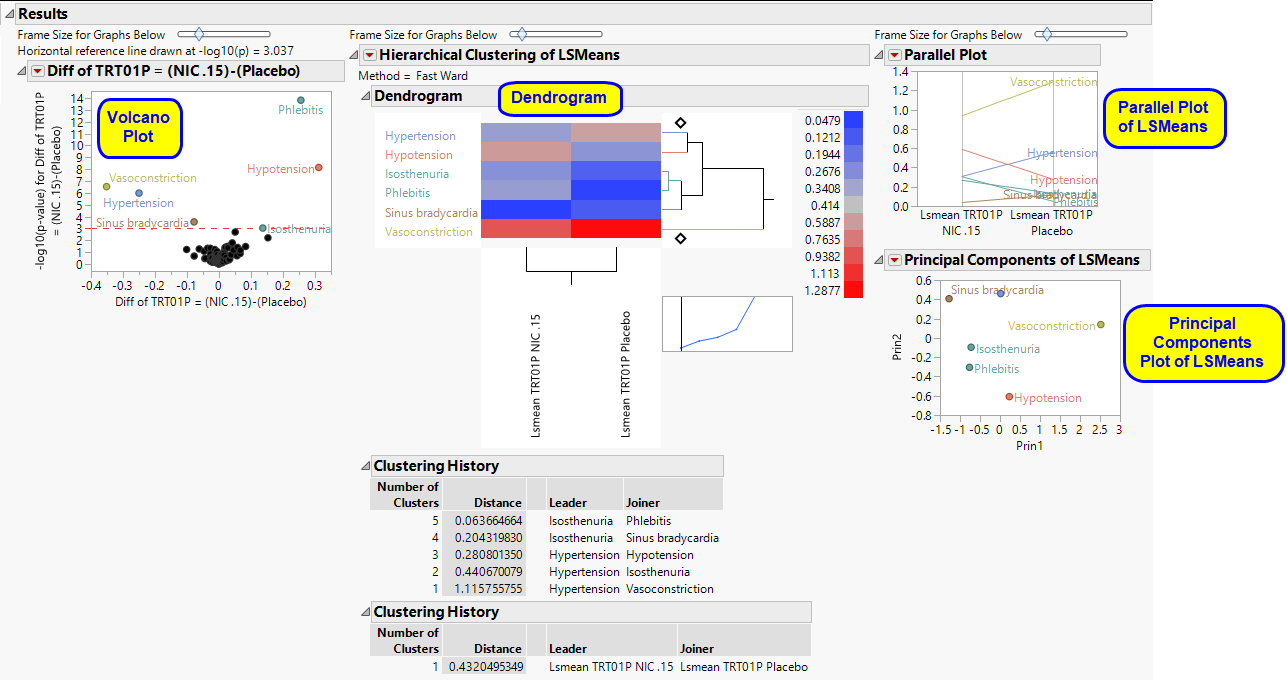
Refer to the LB Results section description for more information about the elements on this section.

The Variability Estimates section contains the results of a distribution and multivariate analysis for each sample.
These show the distributions of each of the variance component estimates from the fitted ANOVA models, including quantiles and summary statistics. You can see which variance components are explaining the most variability across Findings (or adverse event) tests. RSquare is an approximation to the proportion of variability explained by the model. The quantiles can be useful when conducting a power and sample size exercise.
See Distribution for more information.
|
•
|
Multivariate Analysis.
|
These plots provide a multivariate analysis of the variance component estimates, including their correlations and a scatterplot matrix. These reveal interrelationships between the components and how they compete to explain variability.
See Scatterplot Matrix for more information.
|
•
|
Fit Model and Plot LS Means: Select points or rows and click
|
|
•
|
Construct One-way Plots: Click
|
|
•
|
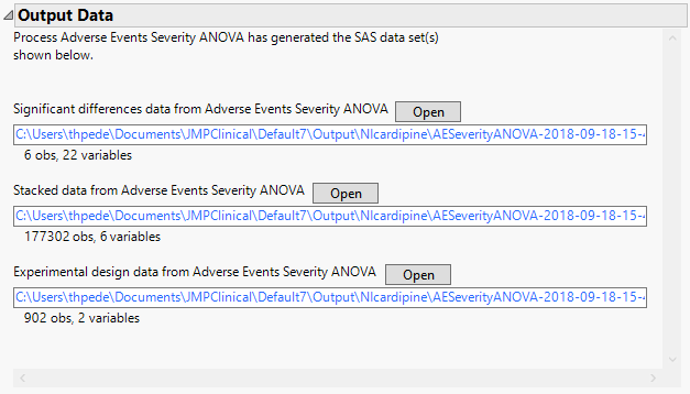
Significant Differences Data Set: This output data set contains a complete list of the adverse events significant by one or more criteria. This data set is indicated by the _sig suffix. Click to view the data set.
|
|
•
|
Stacked Significant Differences Data Set: This output data set contains a complete list of all adverse events for all subjects. It is typically very tall.
|
|
•
|
Experimental Design Data Set: This is a SAS data set that provides information about the columns of a tall data set. It describes relevant experimental variables such as treatment conditions and covariates as well as a variable named ColumnName. Refer to The Example Data for more information. Click to view the data set.
|
|
•
|
Click
|
|
•
|
Click
|
|
•
|
Click
|
|
•
|
Click
|
|
•
|
Click the arrow to reopen the completed report dialog used to generate this output.
|
|
•
|
Click the gray border to the left of the Options tab to open a dynamic report navigator that lists all of the reports in the review. Refer to Report Navigator for more information.
|
Note: For information about how treatment emergent adverse events (TEAEs) are defined in JMP Clinical, please refer to How does JMP Clinical determine whether an Event Is a Treatment Emergent Adverse Event?.
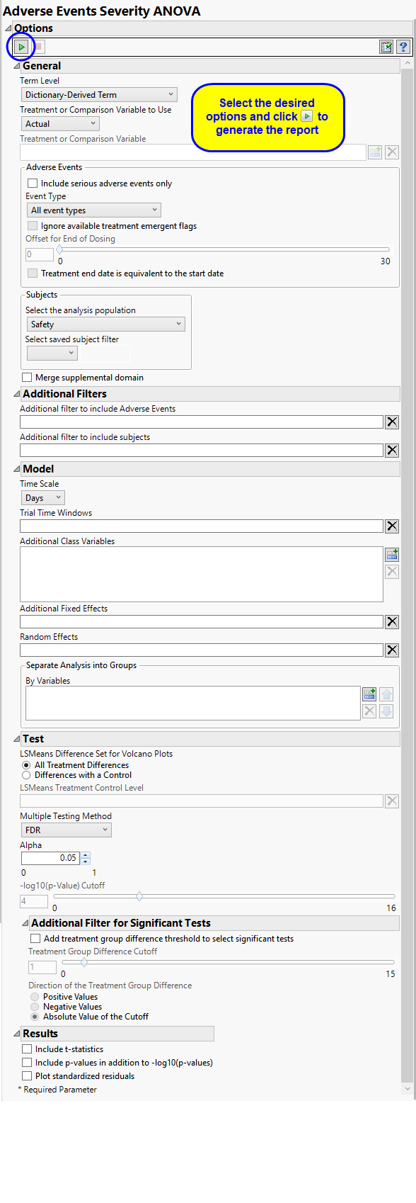
Term Levels are determined by the coding dictionary for the Event or Intervention domain of interest, typically these levels follow the MedDRA dictionary. You must indicate how each adverse event is named and the level at which the event is considered. For example, selecting Reported Term as the Term Level reports the event specified by the actual event term as reported in the AE domain.
The primary goal of clinical trials is to distinguish treatment effects when reporting and analyzing trial results. Treatments are defined by specific values in the treatment or comparison variables of the CDISC models. These variables are specified in this report using the Treatment or Comparison Variable to Use andTreatment or Comparison Variable options.
Available variables include Planned, which is selected when the treatments patients received exactly match what was planned and Actual, which is selected when treatment deviates from what was planned.
You can also specify a variable other than the ARM or TRTxxP (planned treatment) or ACTARM or TRTxxA (actual treatment) from the CDISC models as a surrogate variable to serve as a comparator. Finally you can select None to plot the data without segregating it by a treatment variable.
By default, all events are included in the analysis. However, you can opt to include only those considered serious. Selecting the Include serious adverse events only option restricts the analysis to those adverse events defined as Serious under FDA guidelines.
Analysis can consider all events or only those that emerge at specific times before, during, or after the trial period. For example, selecting On treatment events as the Event Type includes only those events that occur on or after the first dose of study drug and at or before the last dose of drug (+ the offset for end of dosing).
If you choose to Ignore available treatment emergent flags, the analysis includes all adverse events that occur on or after day 1 of the study.
By default, post-treatment monitoring begins after the patient receives the last treatment. However, you might want to specify an Offset for End of Dosing, increasing the time between the end of dosing and post-treatment monitoring for treatments having an extended half-life.
Check the Treatment end date is equivalent to the start date if the treatment end date (EXTENDTC) is missing from the data. In this case, it is assumed that all treatments were given on the same day and that the treatment start date can be used instead.
Filters enable you to restrict the analysis to a specific subset of subjects and/or adverse events based on values within variables. You can also filter based on population flags (Safety is selected by default) within the study data.
If there is a supplemental domain (SUPPAE) associated with your study, you can opt to merge the non-standard data contained therein into your data.
See Select the analysis population, Select saved subject Filter1, Merge supplemental domain, Additional Filter to include Adverse Events, and Additional Filter to Include Subjects for more information.
You can opt to assess interventions across the entire study (specified by default). Alternatively, you can use the Trial Time Windows option to limit it to selected time points or intervals. By default, time is measured in days. However, you can change the Time Scale to measure time in weeks. This option is useful for assessing report graphics for exceptionally long studies.
You can examine the effects that demographics classes have on the occurrence of adverse events by specifying one or more variables using the Additional Class Variables option. Indicator variables are then created for each level of each specified variable.
Use the Additional Fixed Effects option to specify effects by which to model the mean of the response variable. These effects are in addition to the primary time and/or treatment effects, so do not specify any effects confounded with those. The effects can include any mixture of class variables (as specified above) or continuous covariates.
Random Effects are typically comprised of class variables and their interactions that are used to model the covariance structure of the response variable. These effects are in addition to the primary time and/or treatment effects, so do not specify any effects confounded with those. The effects can include any mixture of class variables (as specified above) or continuous covariates. Commonly used random effects are SITEID (for multi-center trials) and STUDYID (for data assembled from multiple studies).
You can also subdivide the subjects and run analyses for distinct groups by specifying one or more By Variables.
LSMeans Difference Set for Volcano Plots Specify the set of lsmeans differences you wish to consider. All Treatment Differences denotes differences between all possible pairs of levels for the Treatment variable. Caution: All Treatment differences can generate numerous differences when there are many levels in your treatment variable. Differences with a Control denotes taking differences against a single reference level that you specify below.
The LSMeans Treatment Control Level is specified as either “Placebo” or “Pbo”, depending on the value found in your data, by default. However, if your control is defined differently you can use the text box to specify the control level is identified in your study.
The False Discovery Rate test is selected by default. You can use the Multiple Testing Method option to select alternative test protocols.
The Alpha option is used to specify the significance level by which to judge the validity of the summary statistics generated by this report. The meaning of alpha depends on the adjustment method that you select. Alpha can be set to any number between 0 and 1, but is most typically set at 0.001, 0.01, 0.05, or 0.10. The higher the alpha, the higher the error rate but also higher the power for detecting significant differences. You will need to decide on the best trade-off for your experiment.
Note that instead of performing multiple testing adjustments of the p-values, you can opt to simply specify a cutoff value for -log10(p-values) in order to select significant hypothesis tests. Using unadjusted p-values with a cutoff has the benefit of more expansive volcano plots, whereas adjusted p-values tend to squish points along the y-axis.Refer to -log10(p-Value) Cutoff for more information. Note: This option is available only when no multiple testing method is specified.
The Add treatment group difference threshold to select significant tests option enables you to use an additional filter based on the magnitude of the treatment group difference (the value that is plotted on the X-axis of the resulting volcano plots) for each statistical test when creating significant indicator variables. This filter, can be used to further highlight clinically interesting results from tests found to be statistically significant. The significant indicator variables formed in the output data set are based on both the p-value cutoff and the magnitude of the treatment group difference specified below.
The Treatment Group Difference Cutoff option enables you to specify a cutoff for the treatment group differences (calculated from the treatment group LSMeans) that are displayed in the X-axis of volcano plots formed for the statistical tests. This cutoff is used to further select significantly interesting hypothesis tests. Note values entered should be positive values indicating the magnitude of the cutoff. Use the Direction of the Treatment Group Difference to specify the direction of the treatment group difference you wish to apply for further selection of significant tests.
Check the Include T-statistics to include extra output columns containing the t-statistics for results from the ESTIMATE statements and LSMEANS differences.
Check the Include p-values in addition to -log10(p-values) option to include extra output columns containing p-values for results from the ESTIMATE statements and LSMEANS differences in addition to the default -log10 p-values.
Residuals are computed as observed dependent variable values minus the predicted values from the anova model. Studying the residuals can help you decide on the validity of the assumptions underlying the anova model, namely, that the errors are approximately normally distributed and independent. The Plot standardized residuals option creates quantile-quantile (Q-Q) and scatter plots of the standardized residuals from the anova model fits. These plots are useful for assessing the quality of each fit. Caution: This option creates a large SAS data set and opens it in JMP for plotting. It can greatly slow execution time for large trials.
Subject-specific filters must be created using the Create Subject Filter report prior to your analysis.