The AE Time to Event report screens all adverse events by performing log-rank and Wilcoxon tests between treatment groups. The time to first occurrence of the adverse event is used as the response.
Note: If you run this analysis using data from a blinded study or from a study that has only one ARM, you generate a different set of output. See AE Time to Event (One ARM) for a detailed description
The AE Time to Event report screens all adverse events by performing log-rank and Wilcoxon tests between treatment groups. The time to first occurrence of the adverse event is used as the response.

Presents summary figures for two popular statistical tests for Kaplan-Meier analyses: the Log-Rank and Wilcoxon.
The Volcano Plots section contains the following elements:
|
•
|
Two Volcano Plots.
|
The Y axis represents the -log10(raw p-value) from either the Log-Rank test (left) or the Wilcoxon test (right). In most instances, these two tests coincide. To interpret this axis, consider the following.
The X axis represents the maximum computed distance between the two curves, and color indicates which treatment was likely to have the event sooner. For example, Phlebitis occurs at approximately 0.27 on the X axis and is green. This means that at least one time point in the Kaplan-Meier and Hazard Plots, the risk of having this particular event was 27% more likely for Nicardipine versus Placebo.
Events above the dotted red line are considered statistically significant after adjusting for multiple comparisons. Adjustment is applied using the linear step-up method of Benjamini and Hochberg (1995) to control the false discovery rate.
See Volcano Plot for more information.
|
•
|
Kaplan-Meier and Hazard Plots: Click
|
|
•
|
Fit Incidence Density Model: Click
|
|
•
|
Click
|
|
•
|
Click
|
|
•
|
Click
|
|
•
|
Click
|
|
•
|
Click the arrow to reopen the completed report dialog used to generate this output.
|
|
•
|
Click the gray border to the left of the Options tab to open a dynamic report navigator that lists all of the reports in the review. Refer to Report Navigator for more information.
|
Note: For information about how treatment emergent adverse events (TEAEs) are defined in JMP Clinical, please refer to How does JMP Clinical determine whether an Event Is a Treatment Emergent Adverse Event?..
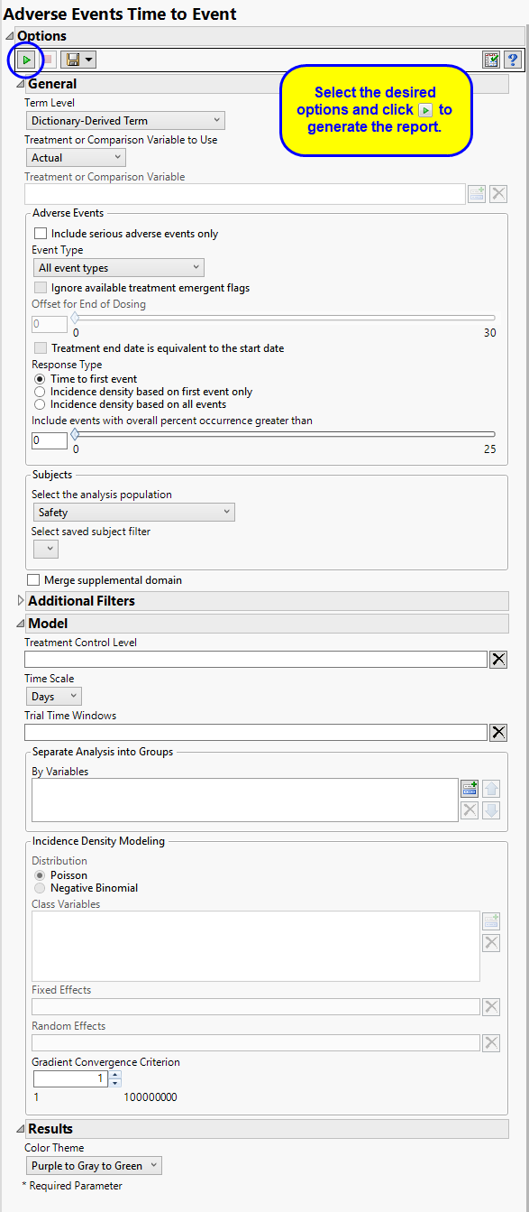
The Term Level is determined by the coding dictionary for the Event or Intervention domain of interest, typically these levels follow the MedDRA dictionary. You must indicate how each adverse event is named and the level at which the event is considered. For example, selecting Reported Term reports the event specified by the actual event term as reported in the AE domain.
The primary goal of clinical trials is to distinguish treatment effects when reporting and analyzing trial results. Treatments are defined by specific values in the treatment or comparison variables of the CDISC models. These variables are specified in this report using the Treatment or Comparison Variable to Use andTreatment or Comparison Variable options.
Available variables include Planned, which is selected when the treatments patients received exactly match what was planned and Actual, which is selected when treatment deviates from what was planned.
You can also specify a variable other than the ARM or TRTxxP (planned treatment) or ACTARM or TRTxxA (actual treatment) from the CDISC models as a surrogate variable to serve as a comparator. Finally, you can select None to plot the data without segregating it by a treatment variable.
By default, all events are included in the analysis. However, you can opt to include only those considered serious. Selecting the Include serious adverse events only option restricts the analysis to those adverse events defined as Serious under FDA guidelines.
Analysis can consider all events or only those that emerge at specific times before, during, or after the trial period. For example, selecting On treatment events as the Event Type includes only those events that occur on or after the first dose of study drug and at or before the last dose of drug (+ the offset for end of dosing).
If you choose to Ignore available treatment emergent flags, the analysis includes all adverse events that occur on or after day 1 of the study.
By default, post-treatment monitoring begins after the patient receives the last treatment. However, you might want to specify an Offset for End of Dosing, increasing the time between the end of dosing and post-treatment monitoring for treatments having an extended half-life.
Check the Treatment end date is equivalent to the start date if the treatment end date (EXTENDTC) is missing from the data. In this case, it is assumed that all treatments were given on the same day and that the treatment start date can be used instead.
By default this report examines the time to the first event as the Response Type, In this analysis, a test of differences of time to first event across treatment groups is conducted using both Log-Rank and Wilcoxon statistics. Alternatively, you can opt to use incidence densities. Incidence densities compare the proportion of occurrences of events across treatment groups. Data for incidence density, based on the first event only, are aggregated to the treatment level whereas data for incidence density based on all events are aggregated to the subject level.
Use the Include events with overall percent occurrence greater than option to specify a threshold for reporting adverse events. Only events that occur above the entered threshold (in terms of overall percent of occurrence) are displayed in the reports. This value is set to 0 by default, so that all adverse event occurrences are included.
Filters enable you to restrict the analysis to a specific subset of subjects and/or adverse events based on values within variables. You can also filter based on population flags (Safety is selected by default) within the study data.
If there is a supplemental domain (SUPPAE) associated with your study, you can opt to merge the non-standard data contained therein into your data.
See Select the analysis population, Select saved subject Filter1, Merge supplemental domain, Additional Filter to include Adverse Events, and Additional Filter to Include Subjects for more information.
The Treatment Control Level is specified as either “Placebo” or “Pbo”, depending on the value found in your data, by default. However, if your control is defined differently you can use the text box to specify the control level is identified in your study.
You can opt to assess interventions across the entire study (specified by default). Alternatively, you can use the Trial Time Windows option to limit it to selected time points or intervals. By default, time is measured in days. However, you can change the Time Scale to measure time in weeks. This option is useful for assessing report graphics for exceptionally long studies.
You can also subdivide the subjects and run analyses for distinct groups by specifying one or more By Variables.
Choose the Distribution the event counts are assumed to follow. Negative binomial fits an extra parameter that can account for over-dispersion.
You can examine the effects that demographics classes have on the occurrence of adverse events by specifying one or more variables using the Class Variables option. Indicator variables are then created for each level of each specified variable.
Specify Fixed Effects by which to model the mean of the response variable. The effects can include any mixture of class variables (as specified above) or continuous covariates. Do not specify the treatment variable as it is automatically included.
Random Effects are typically comprised of class variables and their interactions that are used to model the covariance structure of the response variable. Commonly used random effects are SITEID (for multi-center trials) and STUDYID (for data assembled from multiple studies).
The Gradient Convergence Criterion is a number that is used for determining the convergence for iterations on gradient to numerically solve the GIMMIX model. The specified number here are multiplied by 10-8 and set to NLOPTIONS statement in SAS PROC GLIMMIX.
The Color Theme option enables you to specify the color scheme of the report graphics.
Subject-specific filters must be created using the Create Subject Filter report prior to your analysis.