PROC GLIMMIX Options

Use this parameter to select any options to be added to the PROC GLIMMIX statement.

Available options are listed in the following table:

Option	Definition
ASYCORR	• Displays asymptotic correlation matrix of covariance parameter estimates. It is computed from the corresponding asymptotic covariance matrix (see the description of the ASYCOV option, below)
ASYCOV	• This option requests that the asymptotic covariance matrix of the covariance parameters be displayed. By default, this matrix is the observed inverse Fisher information matrix, which equals 2 H -1, where H is the Hessian (second derivative) matrix of the objective function.
EMPIRICAL	• Computes the estimated variance -covariance matrix of the fixed-effects parameters by using the asymptotically consistent (or sandwich) estimator.
IC=None	• The GLIMMIX procedure normally computes various IC that typically apply a penalty to the (possibly restricted) log likelihood, log pseudo-likelihood, or log quasi-likelihood that depends on the number of parameters and/or the sample size . • Select this option to suppress computation of information criteria (IC) in the "Fit Statistics" table. This is the default for models based on pseudo-likelihoods.
IC=PQ	• The GLIMMIX procedure normally computes various IC that typically apply a penalty to the (possibly restricted) log likelihood, log pseudo-likelihood, or log quasi-likelihood that depends on the number of parameters and/or the sample size. • Select this option to request that the penalties include the number of fixed-effects parameters, when estimation in models with random effects is based on a residual (restricted) likelihood. 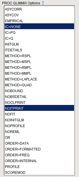Note : For METHOD=MSPL , METHOD=MMPL , METHOD=LAPLACE , and METHOD=QUAD , the IC=Q and IC=PQ options produce the same results.
IC=Q	• The GLIMMIX procedure normally computes various IC that typically apply a penalty to the (possibly restricted) log likelihood, log pseudo-likelihood, or log quasi-likelihood that depends on the number of parameters and/or the sample size. • This is the default option for linear mixed model with normal errors, and the resulting information criteria are identical to the IC option specified using PROC MIXED Options . Note : For METHOD=MSPL , METHOD=MMPL , METHOD=LAPLACE , and METHOD=QUAD , the IC=Q and IC=PQ options produce the same results.
INITGLM	• Requests that the estimates from a generalized linear model fit (a model without random effects) be used as the starting values for the generalized linear mixed model. This option is the default for METHOD=LAPLACE and METHOD=QUAD
ITDETAILS	• Displays the parameter values at each iteration and enables the writing of notes to the SAS log pertaining to infinite likelihood and singularities during Newton-Raphson iterations.
LOGNOTE	• Writes periodic notes to the SAS log describing the current status of computations. • Note : This option was designed for use with analyses requiring extensive CPU resources.
METHOD=RSPL	• Specifies the estimation method in a generalized linear mixed model (GLMM). • The RSPL option specifies that the estimation is based on a R esidual likelihood with a S ubject-specific expansion locus. The PL abbreviation identifies the method as a pseudo-likelihood technique. • This is the default option.
METHOD=MSPL	• Specifies the estimation method in a generalized linear mixed model (GLMM). • The MSPL option specifies that the estimation is based on a M aximum likelihood ( R ) with a S ubject-specific expansion locus. The PL abbreviation identifies the method as a pseudo-likelihood technique.
METHOD=RMPL	• Specifies the estimation method in a generalized linear mixed model (GLMM). • The RMPL option specifies that the estimation is based on a R esidual likelihood with a M arginal-specific expansion locus. The PL abbreviation identifies the method as a pseudo-likelihood technique.
METHOD=MMPL	• Specifies the estimation method in a generalized linear mixed model (GLMM). • The MMPL option specifies that the estimation is based on a M aximum likelihood with a M arginal-specific expansion locus. The PL abbreviation identifies the method as a pseudo-likelihood technique.
METHOD=LAPLACE	• Approximates the marginal likelihood by using Laplace’s method. • Twice the negative of the resulting log -likelihood approximation is the objective function that the procedure minimizes to determine parameter estimates. Laplace estimates typically exhibit better asymptotic behavior and less small-sample bias than pseudo-likelihood estimators. On the other hand, the class of models for which a Laplace approximation of the marginal log likelihood is available is much smaller compared to the class of models to which PL estimation can be applied.
METHOD=QUAD	• Approximates the marginal log likelihood with an adaptive Gauss-Hermite quadrature. • Compared to METHOD=LAPLACE , the models for which parameters can be estimated by quadrature are further restricted.
NOBOUND	• Requests the removal of boundary constraints on covariance parameters. • For example, variance components have a default lower boundary constraint of 0, and the NOBOUND option allows their estimates to be negative.
NOBSDETAIL	• Adds detailed information to the "Number of Observations" table to reflect how manySuzanne Fields were excluded from the analysis and for which reason.
NOCLPRINT	• Suppresses the display of the Class Level Information table if you do not specify number. • If you do specify number, only levels with totals that are less than number are listed in the table.
NOITPRINT	• Suppresses the display of the Iteration History table.
NOFIT	• Suppresses fitting of the model.
NOINITGLM	• Requests that the starting values for the fixed effects not be obtained by first fitting a generalized linear model. • This option is the default for the pseudo-likelihood estimation methods and for the linear mixed model. For the pseudo-likelihood methods, starting values can be implicitly defined based on an initial pseudo-data set derived from the data and the link function. For linear mixed models, starting values for the fixed effects are not necessary.
NOPROFILE	• Includes the residual variance as part of the Newton-Raphson iterations. • This option applies only to models that have a residual variance parameter. • By default, this parameter is profiled out of the likelihood calculations.
NOREML	• Determines the denominator for the computation of the scale parameter in a GLM for normal data and for overdispersion parameters. • In GLMM models fit by pseudo-likelihood methods, the NOREML option changes the estimation method to the nonresidual form.
OR	• Requests that odds ratios be added to the output when applicable.
ORDER=DATA	• Specifies that the levels of the classification variables are sorted in the order in which they appear in the input data set.
ORDER=FORMATTED	• Specifies that the levels of the classification variables are sorted in the order specified by an external formatted variable.
ORDER=FREQ	• Specifies that the levels of the classification variables are sorted in the order of descending frequency count.
ORDER=INTERNAL	• Specifies that the levels of the classification variables are sorted in the order specified by an unformatted variable.
PROFILE	• Requests that scale parameters be profiled from the optimization, if possible. • This is the default for generalized linear mixed models. Note : In generalized linear models with normally distributed data, you can use the PROFILE option to request profiling of the residual variance.
SCOREMOD	• Requests that the Hessian matrix in GLMMs be based on a modified scoring algorithm, provided that PROC GLIMMIX is in scoring mode when the Hessian is evaluated.

To Specify One or More PROC GLIMMIX Options:

Left-click on the desired option.

To specify more than one option, hold down Ctrl as you left-click on the desired options.

Refer to the SAS PROC GLIMMIX documentation for more information and references.