SAS Code for Generating JSL

Let us now consider the SAS code that generates JSL for the Distribution Analysis process. This code is located in the ProcessLibrary folder in your JMP installation directory.

Navigate to the ProcessLibrary folder.

Open the DataDistribution.sas file using a text editor.

Scroll towards the bottom of the file.

The code used to generate the JSL is found towards the end of the SAS code.

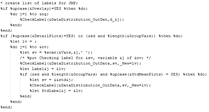
This section of the Distribution Analysis SAS code begins ( Figure ) by invoking the %CheckLabel macro in a loop across all specified variables in the Vars macro. This creates new macro variables that contain the SAS labels for these variables, and these variables are then referenced in subsequent PUT statements.

The code then defines the file in which to place the JSL code via a %PrepOutFile macro, which issues a FILENAME statement corresponding to the .jsl file to be created, referenceable with the DataDistributionScript macro variable ( Figure ).

The principal part of the code (partially shown below) is contained within a DATA _NULL_ block, which contains a series of PUT statements to push individual lines of JSL code to the previously created file. This approach allows you to exploit the power of the SAS macro language to automatically create all of the displays and analyses that you want in JMP. You can also use looping and macro referencing to make your code generic enough to run on any data set of a similar structure.

In this example, the first JSL line “//!" (line 4 of the code illustrated above) instructs JMP to automatically run the script. Following the initial setup of tabbed windows, if the user has requested overlaid kernel density estimates, an Open statement tells JMP to open the densities SAS data set as a JMP table. (This SAS data set was created in an earlier part of the code using PROC KDE.). The next JSL commands color and label the rows in the resulting JMP table. Then the JMP Parallel Plot platform is called to show the colored densities. A double macro reference &&_&j is used in a loop to dereference macro variables _1, _2, _3, … which correspond to density values along the x axis. A similar pattern is followed in subsequent PUT statements for the box plots and distribution analyses (code not shown) as shown in the previous JMP displays.

Probably the most difficult aspect of writing code such as this involves appropriate punctuation, especially when generating JSL code that contains special characters such as quotation marks. You should review the documentation for the PUT statement in Base SAS software and the Macro Quoting documentation in SAS Macro Language to make sure you are setting up your code correctly. Of course studying and working from examples like this one is also an effective way to start creating your own code.

Note that some PUT statements use double quotes, whereas others use single quotes. Single quotes are desirable in cases where the line is a static literal string and contains special characters like embedded double quotes. The disadvantage of using single quotes is that no macro variable substitution is performed within them. Double quoted PUT strings do allow macro variable substitution, but then special care is needed to create embedded double quotes as needed in many JSL commands like Open and New Window . Make sure to end each PUT statement with a semicolon, and try to include extra lines and leading spaces so that the generated JSL code is well-formatted.

The SAS macro language can sometimes generate unusual error messages when quotation marks are unbalanced or misaligned. If you encounter such messages, it can be helpful to adopt a divide-and-conquer strategy for your code by commenting out parts of the code using /* */ blocks and making sure that each uncommented part works correctly before putting the parts back together.

Both the parallel plot and distribution code involve loops through different sets of variables. The parallel plot variables come from the density estimation process and this data set is transposed so that each curve is a selectable row in the plot. The variables in the distribution analysis are just the originally specified variables, although, as mentioned earlier, their labels are used rather than the variable names themselves. The labels are inserted in the JSL code with the &&Label&j macro specification.

The SAS code finishes with instructions to run the process and include specific output files in the output folder (below).

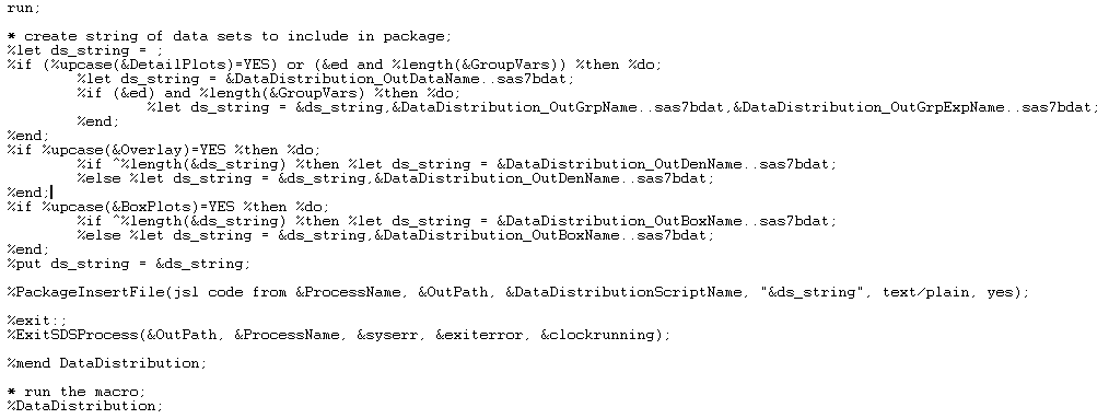
The generated .jsl file is included in the SAS package via the %PackageInsertFile macro. JMP Life Sciences recognizes the .jsl suffix in the package and automatically launches the JSL code after the SAS job finishes.

Next : Macros Available for JMP Life Sciences Processes