Example of the Degradation Platform

This example uses the GaAs Laser.jmp data table from Meeker and Escobar (1998), which contains measurements of the percent increase in operating current taken on several gallium arsenide lasers. When the percent increase reaches 10%, the laser is considered to have failed.

Select Help > Sample Data Library and open Reliability/GaAs Laser.jmp.

Select Analyze > Reliability and Survival > Degradation.

Select Current and click Y, Response.

Select Hours and click Time.

Select Unit and click Label, System ID.

Type 10 in the text box for Upper Spec Limit.

Click OK.

Initial Degradation Report

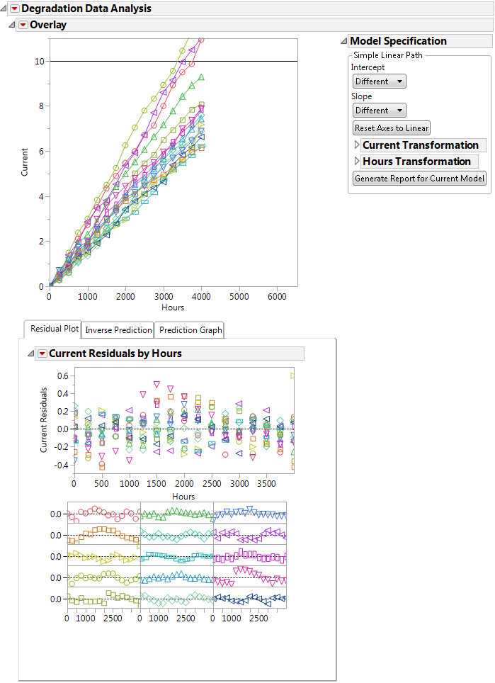
Initial Degradation Report shows the initial Degradation report. The Overlay plot shows the measurements of Current versus Time for each unit in the data. The horizontal line at Current = 10 corresponds to the upper specification limit at 10%. Units with values above this limit are considered to have failed. Three of the fifteen units have reached that point by the end of the study period. The Inverse Prediction outline shows the predicted Hours value for which each unit fails, based on your specified model.

The default model fits a separate slope and intercept for each unit, using linear transformations. You can fit other models using the Model Specification outline.

The Residual Plot tab in Initial Degradation Report shows residuals based on your specified model. The top plot shows residuals for all units plotted against Hours and overlaid on one plot. The bottom plot shows individual plots of the residuals for each unit in a rectangular array.