Example of the Save Discrim Option | JMP 13.2

JMP Support 800.450.0135 (US)

Documentation Feedback
Your feedback is important to us. us any comments about our documentation.

Fitting Linear Models • Multivariate Response Models • Discriminant Analysis • Example of the Save Discrim Option

•

Example of the Save Discrim Option

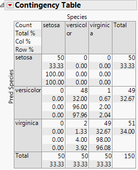
Examine Fisher’s Iris data as found in Mardia, Kent, and Bibby (1979). There are k = 3 levels of species and four measures on each sample.

1.

Select Help > Sample Data Library and open Iris.jmp.

2.

Select Analyze > Fit Model.

3.

Select Sepal length, Sepal width, Petal length, and Petal width and click Y.

4.

Select Species and click Add.

5.

Next to Personality, select Manova.

6.

7.

From the red triangle menu next to Manova Fit, select Save Discrim.

The following columns are added to the Iris.jmp sample data table:

Quadratic form needed in the Mahalanobis distance calculations.

Mahalanobis distance of the observation from the Setosa centroid.

SqDist[versicolor]

Mahalanobis distance of the observation from the Versicolor centroid.

SqDist[virginica]

Mahalanobis distance of the observation from the Virginica centroid.

Sum of the negative exponentials of the Mahalanobis distances, used below.

Probability of being in the Setosa category.

Prob[versicolor]

Probability of being in the Versicolor category.

Prob[virginica]

Probability of being in the Virginica category.

Species that is most likely from the probabilities.

Now you can use the new columns in the data table with other JMP platforms to summarize the discriminant analysis with reports and graphs. For example:

1.

From the updated Iris.jmp data table (that contains the new columns) select Analyze > Fit Y by X.

2.

Select Species and click Y, Response.

3.

Select Pred Species and click X, Factor.

4.

The Contingency Table summarizes the discriminant classifications. Three misclassifications are identified.

Contingency Table of Predicted and Actual Species

•

Help created on 9/19/2017