To model nonlinear degradation paths, select Degradation Path Style > Nonlinear Path from the platform red triangle menu. This is useful if a degradation path cannot be linearized using transformations, or if you have a custom nonlinear model that you want to fit to the data.
To facilitate explaining the Nonlinear Path Model Specification, open the Device B.jmp data table. The data consists of power decrease measurements taken on 34 units, across four levels of temperature. Follow these steps:
|
1.
|
|
2.
|
|
3.
|
|
4.
|
|
5.
|
|
6.
|
|
7.
|
Click OK.
|
Device B Overlay Plot shows the initial overlay plot of the data.

The degradation paths appear linear for the first several hundred hours, but then start to curve. To fit a nonlinear model, select Degradation Path Style > Nonlinear Path from the platform red triangle menu to show the Nonlinear Path Model Specification outline. See Initial Nonlinear Model Specification Outline.
Note: To view the Edit button displayed in Initial Nonlinear Model Specification Outline, you must have the interactive formula editor preference selected (File > Preferences > Platforms > Degradation > Use Interactive Formula Editor).
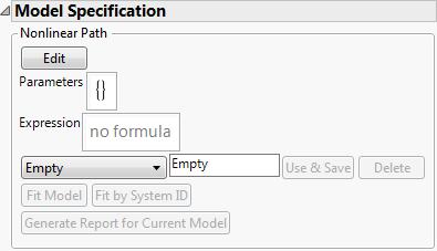
The first step to create a model is to select one of the options on the menu initially labeled Empty:
The Reaction Rate options are applicable when the degradation occurs from a single chemical reaction, and the reaction rate is a function of temperature only. Select Reaction Rate or Reaction Rate Type 1 from the menu shown in Initial Nonlinear Model Specification Outline. Although similar to the Reaction Rate model, the Reaction Rate Type 1 model contains an offset term that changes the basic assumption concerning the response value’s sign.
For this example, select Reaction Rate and then select Celsius as the Temperature Unit. Click OK to return to the report. For details about all the features for Model Specification, refer to Model Specification Details.
Select Constant Rate from the menu shown in Initial Nonlinear Model Specification Outline. The Constant Rate Model Settings window prompts you to enter transformations for the Path, Rate, and Time.
Once a selection is made for each transformation, the associated formula appears in the lower left corner as shown in Constant Rate Transformation.
After all selections are made, click OK to return to the report. For details about all the features for Model Specification, refer to Model Specification Details.
For details about how to create a custom model and store it as a column formula, refer to Fit a Custom Model or Nonlinear Regression in the Predictive and Specialized Modeling book.
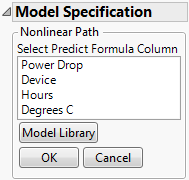
Select Prediction Column from the list that appears beneath the Expression area in Initial Nonlinear Model Specification Outline. The Model Specification outline changes to prompt you to select the column that contains the model.
|
•
|
If the model that you want to use already exists as a formula in a column of the data table, select the corresponding column here, and then click OK. You are returned to the Nonlinear Path Model Specification. For details about all the features for that specification, refer to Model Specification Details.
|
|
•
|
If the model that you want to use does not already exist in the data table, you can click the Model Library button to use one of the built-in models. For details about using the Model Library button, refer to Model Library or Nonlinear Regression in the Predictive and Specialized Modeling book. After the model is created, select Redo > Redo Analysis from the Degradation Data Analysis red triangle menu. Then, return to the column selection shown in Column Selection. Select the column that contains the model, and then click OK. You are returned to the Nonlinear Path Model Specification. For details about all the features for that specification, refer to Model Specification Details.
|
|
•
|
If the model that you want to use is not in the data table, and you do not want to use one of the built-in models, then you are not ready to use this model specification. First, create the model, relaunch the Degradation platform, and then return to the column selection (Column Selection). Select the column containing the model, and then click OK. You are returned to the Nonlinear Path Model Specification. For details about all the features for that specification, refer to Model Specification Details.
|
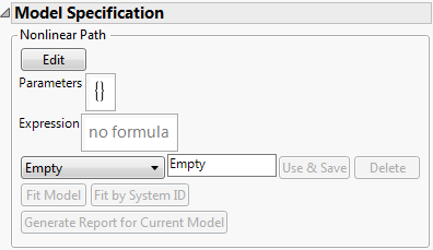
Note: To view the Edit button displayed in Model Specification, you must have the interactive formula editor preference selected (File > Preferences > Platforms > Degradation > Use Interactive Formula Editor).
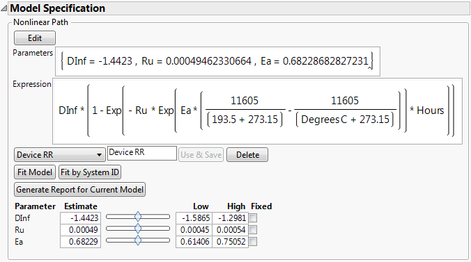
A model is now shown in the script box that uses the Parameter statement. Initial values for the parameters are estimated from the data. For complete details about creating models that use parameters, refer to Fit a Custom Model or Nonlinear Regression in the Predictive and Specialized Modeling book.
If desired, type a name in the text box to name the model. For this example, use the name “Device RR”. After that, click the Use & Save button to enter the model and activate the other buttons and features. Model Specification shows the Model Specification window after clicking the Use & Save button.
|
•
|
The Fit Model button is used to fit the model to the data.
|
|
•
|
|
•
|
The Delete button is used to delete a model from the model menu.
|
|
•
|
The Generate Report for Current Model button creates a report for the current model settings. See Model Reports.
|
The initial parameter values are shown at the bottom, along with sliders for visualizing how changes in the parameters affect the model. To do so, first select Graph Options > Show Fitted Lines from the platform red-triangle menu to show the fitted lines on the plot. Then move the parameter sliders to see how changes affect the fitted lines.
|
•
|
 ) - asymptotic degradation level
|
•
|
|
•
|
Ea (Ea) - reaction-specific activation energy
|
 x {1-exp[-
where RU is the reaction rate at use temperature tempU, RU x AF(temp) is the reaction rate at a general temperature temp, and for temp > tempU, AF(temp) > 1
AF(temp) =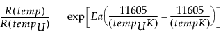
To fix a value for a parameter, check the box under Fixed for the parameter. When fixed, that parameter is held constant in the model fitting process.
You can use the Formula Editor to enter a model. Click the Edit button to open the Formula Editor to enter parameters and the model. For details about entering parameters and formulas in the Formula Editor, see Formula Editor in the Using JMP book.
Note: To view the Edit button displayed in Alternate Model Specification Report, you must have the interactive formula editor preference selected (File > Preferences > Platforms > Degradation > Use Interactive Formula Editor).
|
4.
|
Select Parameters from the list in the lower left corner.
|
|
5.
|
Click New Parameter.
|
|
9.
|
Click OK.
|
In the formula editor, when you add a parameter, note the check box for Expand Into Categories, selecting column. This option is used to add several parameters (one for each level of a categorical variable for example) at once. When you select this option a window appears that enables you to select a column. After selection, a new parameter appears in the Parameters list with the name D_column, where D is the name that you gave the parameter. When you use this parameter in the formula, a Match expression is inserted, containing a separate parameter for each level of the grouping variable.
Model Library
The Model Library can assist you in creating a formula column with parameters and initial values. Click Model Library under Model Specification to open the library. Select a model in the list to see its formula in the Formula box.
Click Show Graph to show a 2-D theoretical curve for one-parameter models and a 3-D surface plot for two-parameter models. No graph is available for models with more than two explanatory (X) variables. Use the slider bars to change the default starting values for the parameters. You can also click on the values and enter new values directly.
The Reset button sets the starting values for the parameters back to their default values.
Click Show Points to overlay the actual data points to the plot. A window opens, asking you to assign columns into X and Y roles, and an optional Group role. The Group role allows for fitting the model to every level of a categorical variable. If you specify a Group role here, also specify the Group column on the platform launch window.
Click Make Formula to create a new column in the data table. This column has the formula as a function of the specified X variable and uses the parameter values specified in the graph window.
Note: If you click Make Formula before you click the Show Graph or Show Points buttons, you are asked to provide the X and Y roles, and an optional Group role. After that, you are brought back to the plot so that you have the option to adjust the starting values for the parameters. Once the starting values for the parameters are satisfactory, click Make Formula again to create the new column.
Once the formula is created in the data table, select Redo > Redo Analysis from the Degradation Data Analysis red triangle menu. Then, return to the column selection shown in Column Selection. Select the column that contains the model, and then click OK. You are returned to the Nonlinear Path Model Specification. For details about all the features for that specification, refer to Model Specification Details.
Note: You can customize the models included in the Nonlinear Model Library by modifying the built-in script named NonlinLib.jsl. This script is located in the Resources/Builtins folder in the folder that contains JMP (Windows) or in the Application Package (Macintosh).