This example of an accelerated destructive degradation model is patterned after an example from Escobar et al. (2003). The data consist of measurements on the strength (measured in newtons) of an adhesive bond. Temperature is considered to be an acceleration factor. The product is stressed until the bond breaks and the required breaking stress is recorded. Because units at normal use conditions are unlikely to break, the units were tested at several levels over a wide range of temperatures. Strength less than 50 newtons is considered failure. You want to estimate the proportion of units with a strength below 50 newtons after 260 weeks (5 years) at use conditions of 35 degrees Celsius.
|
1.
|
|
2.
|
|
3.
|
|
4.
|
|
5.
|
|
6.
|
Notice that the Censor Code is set to Right.
|
7.
|
Click OK.
|
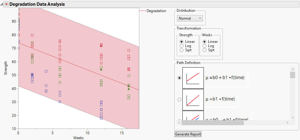
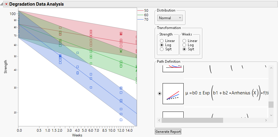
Figure 7.2 Initial Degradation Plot
|
1.
|
|
2.
|
|
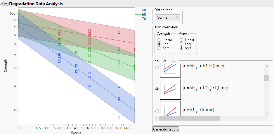
3.
|
The subscript “x” denotes the accelerating variable, which is Degrees in this example.
Figure 7.3 Plot Showing Model
|
4.
|
Click Generate Report.
|
Figure 7.4 Report for Basic Model
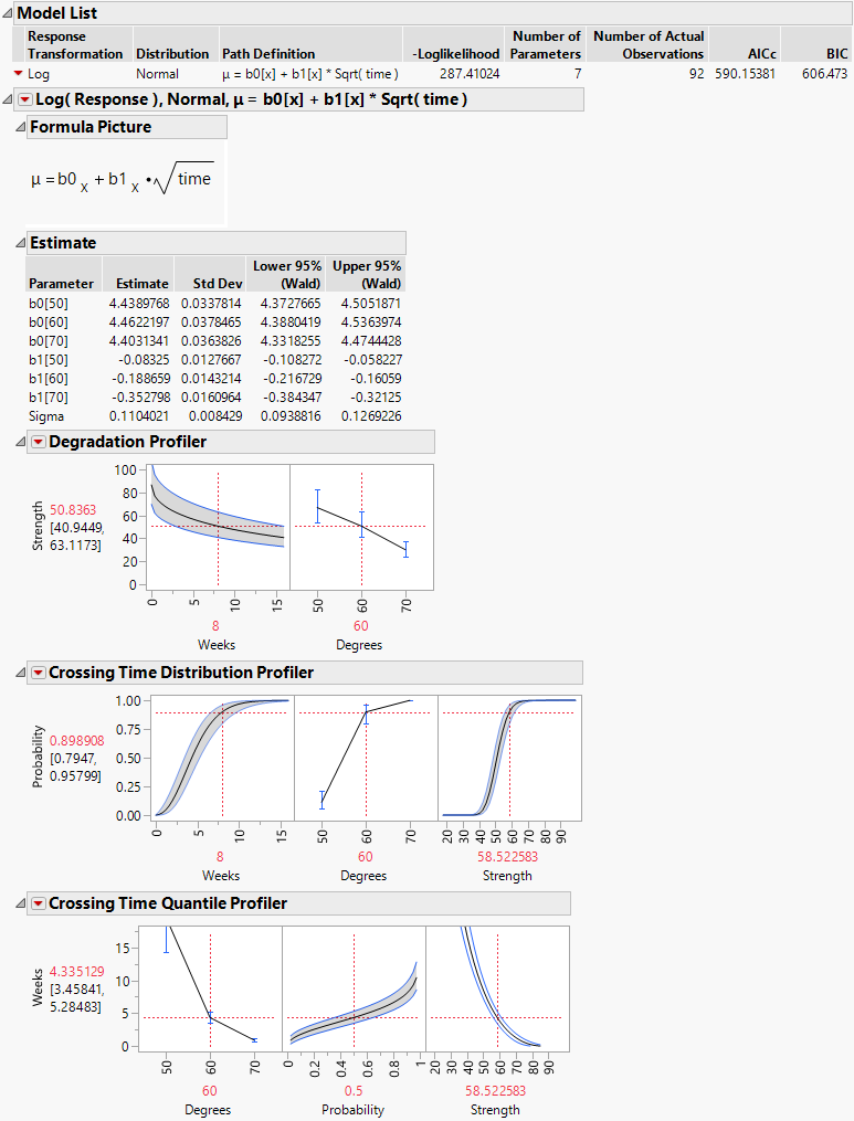
The estimates of the slope b1 at the three values of Degrees suggest that degradation occurs more quickly at higher temperatures. Failure mechanisms that depend on chemical processes are often well modeled using the Arrhenius model for temperature. For this reason, you now fit a model where an Arrhenius transformation is applied to Degrees, which is measured on a Celsius scale.
|
5.
|
Select μ = b0 ± Exp(b1 + b2*Arrhenius(X))*f(time) for the Path Definition.
|
|
6.
|
|
7.
|
Click Generate Report.
|
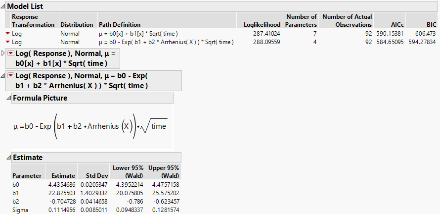
Because the Arrhenius model shows a better fit, as indicated by its smaller AICc and BIC values (Figure 7.6), you continue your analysis using this model.
|
1.
|
Figure 7.7 Degradation Profiler
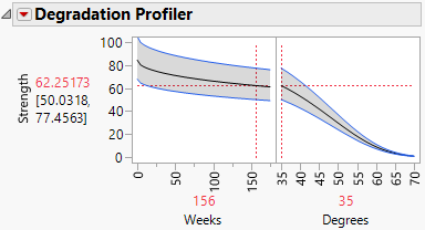
The predicted Strength at these settings is 62.25173, with a 95% prediction interval ranging from 50.0318 to 77.4563. Failures are not very likely at these or less extreme settings.
|
2.
|
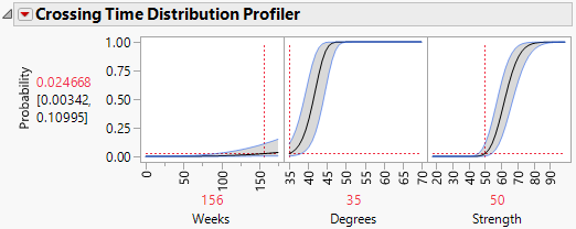
Figure 7.8 Crossing Time Distribution Profiler
|
3.
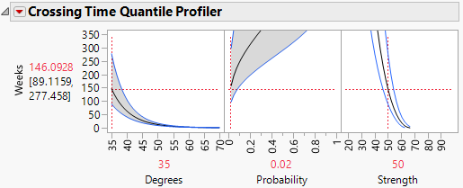
|
Figure 7.9 Crossing Time Quantile Profiler