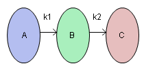
This example is adapted from Box and Draper (2007) and uses Stochastic Optimization.jmp. A chemical reaction converts chemical A into chemical B and B into C. The resulting amount of chemical B is a function of reaction time and reaction temperature. Use the profiler and simulator to explore factor settings to optimize the yield of B.
Figure 8.13 Chemical Reaction
For this reaction the yield of B can be computed using the Arrhenius laws. The column Yield contains the formula for yield. The formula is a function of Reaction Time (hours) and reaction rates k1 and k2. The reaction rates are a function of Reaction Temperature (degrees Kelvin) and known physical constants θ1, θ2, θ3, θ4. Therefore, Yield is a function of Reaction Time and Reaction Temperature.
|
1.
|
|
2.
|
Select Graph > Profiler.
|
|
3.
|
|
4.
|
The Prediction Profiler with Desirability Functions enabled appears. For more information about Desirability Functions, see the Desirability Profiling and Optimization in Profiler.
|
5.
|
Click the Prediction Profiler red triangle and select Optimization and Desirability > Maximize Desirability.
|
The Prediction Profiler maximizes Yield and sets the graphs to the optimum value of Reaction Time and Reaction Temperature.
Figure 8.14 Yield Maximum
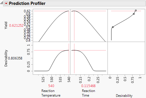
The maximum Yield is approximately 0.62 at a Reaction Time of 0.115 hours and Reaction Temperature of 540 degrees Kelvin, or hot and fast. (Your results might differ slightly due to random starting values in the optimization process.)
In a production environment, process inputs cannot always be controlled exactly. What happens to Yield if the inputs (Reaction Time and Reaction Temperature) have random variation? Furthermore, if Yield has a spec limit, what percent of batches are out of spec? The Simulator can help you investigate the variation and defect rate for Yield, given variation in Reaction Time and Reaction Temperature.
|
1.
|
Click the Prediction Profiler red triangle and deselect Optimization and Desirability > Desirability Functions.
|
|
2.
|
|
3.
|
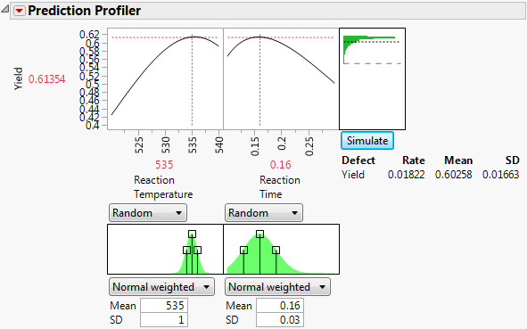
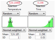
Set the simulation parameters for Reaction Temperature to Random > Normal Weighted with Mean = 540 and SD = 1.
|
|
4.
|
Set the simulation parameters for Reaction Time to Random > Normal Weighted with Mean = 0.115 and SD = 0.03.
|
|
5.
|
Set the N Runs value to 15,000.
|
Figure 8.15 Initial Simulator Settings
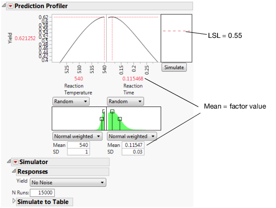
Yield has a lower spec limit of 0.55, set as a column property, and shows in Figure 8.15 as a dashed red line.
|
6.
|
Click the Simulate button.
|
Note: Your numbers might differ from those shown in Figure 8.16 due to the random draws in the simulation.
Figure 8.16 Simulation Results
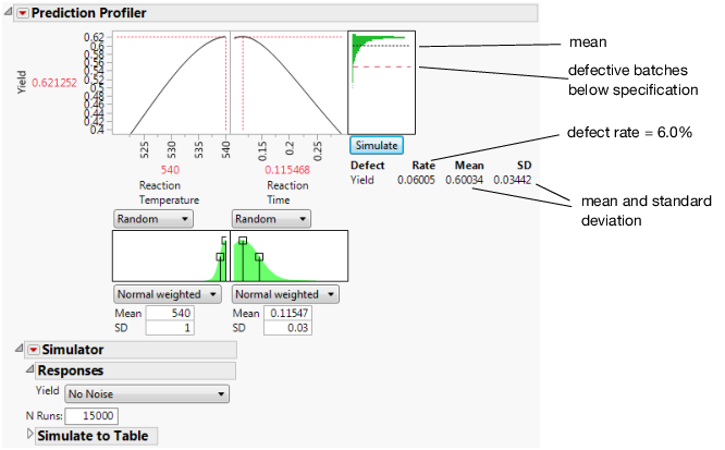
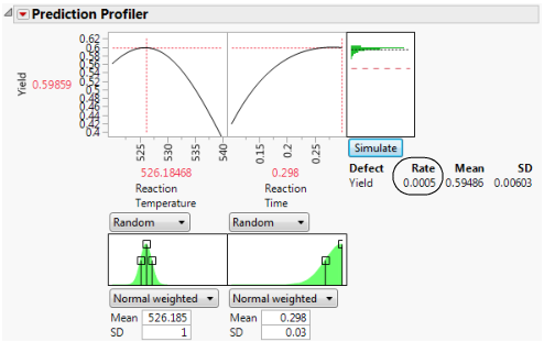
The predicted Yield is 0.62 for Reaction Temperature of 540 and Reaction Time of 0.115. The simulation estimates an average defect rate of about 6% with a standard deviation of 0.03 given the assumed variation in the temperature and time. The defect rate of 6.0%, indicates that about 6.0% of batches would be out of specification.
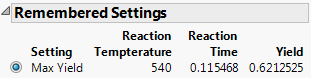
Use the simulator to explore other settings of Reaction Temperature and Reaction Time that might maintain a high Yield but with a lower defect rate. Before changing settings, save these factor settings that give us the maximum Yield for later use.
|
7.
|
Click the Prediction Profiler red triangle and select Factor Settings > Remember Settings.
|
|
8.
|
|
9.
|
Set the Mean value for Reaction Temperature to 535.
|
Using the dashed red line in the Reaction Time plot, you can explore and determine the approximate value that maximized Yield. This value should be around 0.16.
|
10.
|
Set the Mean value of Reaction Time to 0.16.
|
|
11.
|
Click Simulate.
|
Note: Your numbers might differ from those shown in Figure 8.18 due to the random draws in the simulation.
By making slight changes to the input factor settings, the defect rate decreases to about 1.8% with a decrease of less than 0.01 in the predicted yield. The fixed (no variability) settings that maximize Yield are not the same settings that minimize the defect rate in the presence of factor variation.
You can run a simulation experiment to find the settings of Reaction Temperature and Reaction Time that minimize the defect rate. To do this, simulate the defect rate at each point in an experimental design for Reaction Temperature and Reaction Time. Then fit a predictive model for the defect rate and find factor settings to minimize the defect rate.
|
1.
|
|
3.
|
Click OK.
|
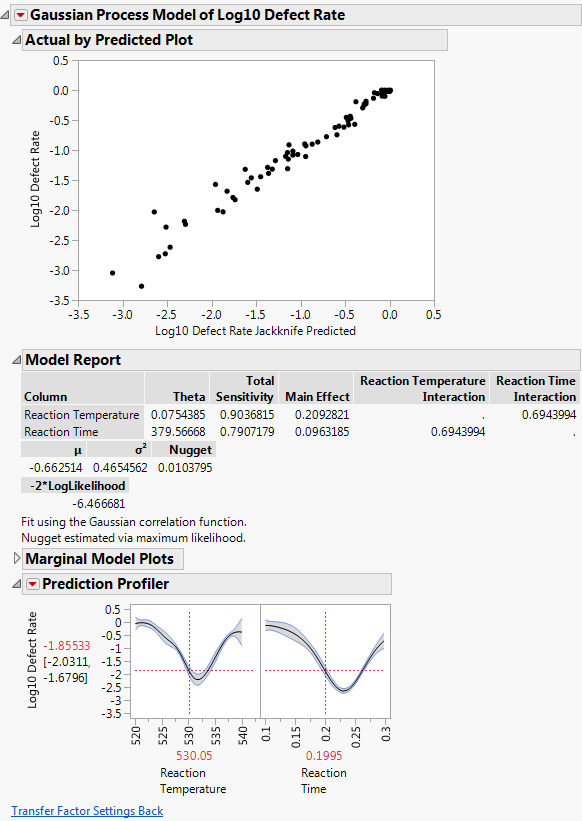
A data table is created with the results of the experiment. The Overall Defect Rate is given at each design point. You can now fit a model that predicts the defect rate as a function of Reaction Temperature and Reaction Time.
Figure 8.19 Results of Gaussian Process Model Fit
|
5.
|
To find the settings of Reaction Temperature and Reaction Time that minimizes the defect rate, click the Prediction Profiler red triangle and select Optimization and Desirability > Maximize Desirability.
|
Figure 8.20 Settings for Minimum Defect Rate
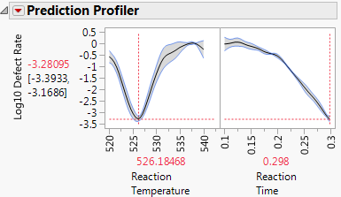
The settings that minimize the defect rate are approximately Reaction Temperature = 526 and Reaction Time = 0.3.
|
6.
|
Click the Transfer Factor Settings Back button.
|
This updates the original Profiler report to use the setting for Reaction Temperature and Reaction Time that minimize the defect rate.
|
8.
|
Click the Prediction Profiler red triangle and select Factor Settings > Remember Settings.
|
|
9.
|
Figure 8.21 Minimum Defect Settings
|
10.
|
With the new settings in place, click the Simulate button to estimate the defect rate at the new settings.
|
Figure 8.22 Lower Defect Rate
At the new settings the defect rate is 0.05%. This is much lower than the 6.0% for the settings that maximize Yield. That is a reduction of about 120x. Recall that the average Yield from the first settings is 0.62, and the new average is 0.59. The decrease in average Yield of 0.03 is the trade off for lowering the defect rate by 120x.
|
11.
|
Click the Remembered Settings radio buttons to view the profiler for each setting.
|
Figure 8.23 Settings Comparison
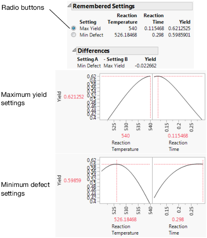
The chemist now knows what settings to use for a quality process. If the factors have no variation, the settings for maximum Yield are hot and fast. But, if the process inputs have variation similar to what we have simulated, the settings for maximum Yield produce a high defect rate. Therefore, to minimize the defect rate in the presence of factor variation, the settings should be cool and slow.