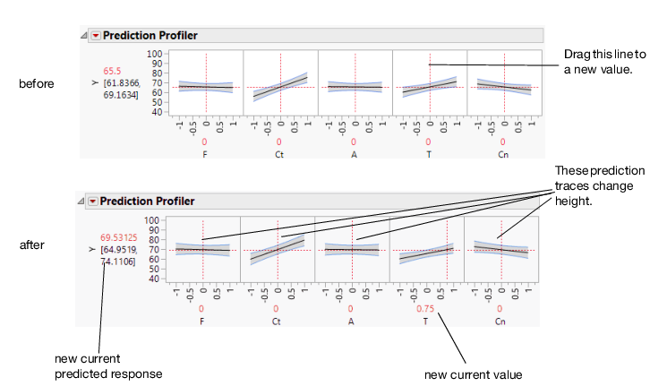
The illustration in Figure 2.4 describes how to use the components of the Prediction Profiler. There are several important points to note when interpreting a prediction profile:
|
•
|
If you change the value of a factor, the prediction trace for that factor is not affected, but the prediction traces of all the other factors can change. The Y response line must cross the intersection points of the prediction traces with their current value lines.
|
Figure 2.4 Changing One Factor from 0 to 0.75
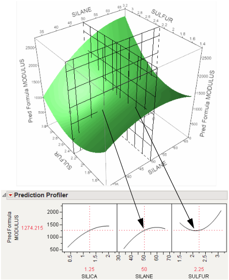
In the following example using Tiretread.jmp, look at the response surface of the expression for MODULUS as a function of SULFUR and SILANE (holding SILICA constant). Now look at how a grid that cuts across SILANE at the SULFUR value of 2.25. Note how the slice intersects the surface. If you transfer that down below, it becomes the profile for SILANE. Similarly, note the grid across SULFUR at the SILANE value of 50. The intersection when transferred down to the SULFUR graph becomes the profile for SULFUR.
Figure 2.5 Profiler as a Cross-Section
Now consider changing the current value of SULFUR from 2.25 to 1.5.
Figure 2.6 Profiler as a Cross-Section
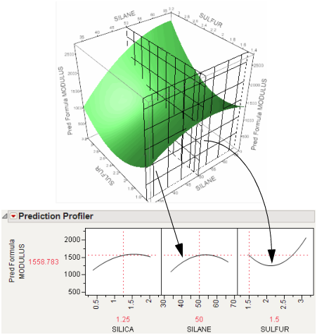
In the Prediction Profiler, note the new value just moves along the same curve for SULFUR, the SULFUR curve itself does not change. But the profile for SILANE is now taken at a different cut for SULFUR. The profile for SILANE is also a little higher and reaches its peak in the different place, closer to the current SILANE value of 50.
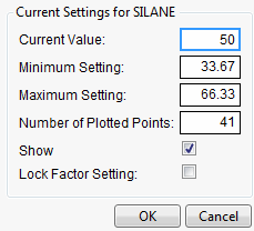
Figure 2.7 Continuous Factor Settings Window