Either a single number that designates the number of desired knot points based on percentiles of x or a vector of values that designate the internal knot points.
Returns values of the empirical cumulative probability distribution function for Y, which can be a vector or a list. Cumulative probability is the proportion of data values less than or equal to the value of QuantVec.
{QuantVec, CumProbVec} = CDF(YVec)
If L is the Cholesky root of an nxn matrix A, then after calling cholUpdate L is replaced with the Cholesky root of A+V*C*V' where C is an mxm symmetric matrix and V is an n*m matrix.
Calculates the correlation matrix of the data in the matrix argument.
A matrix that contains the data. If the data has m rows and n columns, the result is an m-by-m matrix.
Calculates the covariance matrix of the data in the matrix argument.
A matrix that contains the data. If the data has m rows and n columns, the result is an m-by-n matrix.
Creates a design matrix that contains a column of 1s and 0s for each unique value of a vector of values.
An optional argument that changes the handling of values in the vector argument that do not appear in the levelsList argument. If this argument is specified, missing values are placed in the design matrix. Otherwise, 0s are placed in the design matrix.
Missing values in the levelsList argument are not ignored. For example:
Show( Design ( ., [. 0 1] ),
Design( 0, [. 0 1] ),
Design( 1, [. 0 1] ),
Design( [0 0 1 . 1], [. 0 1] ),
Design( {0, 0, 1, ., 1}, [. 0 1] ) );
Design(., [. 0 1]) = [1 0 0];
Design(0, [. 0 1]) = [0 1 0];
Design(1, [. 0 1]) = [0 0 1];
Design([0 0 1 . 1], [. 0 1]) =
[ 0 1 0,
0 1 0,
0 0 1,
1 0 0,
0 0 1];
Design({0, 0, 1, ., 1}, [. 0 1]) =
[ 0 1 0,
0 1 0,
0 0 1,
1 0 0,
0 0 1];
An optional argument that changes the handling of values in the vector argument that do not appear in the levelsList argument. If this argument is specified, missing values are placed in the design matrix. Otherwise, 0s are placed in the design matrix.
An optional argument that changes the handling of values in the vector argument that do not appear in the levelsList argument. If this argument is specified, missing values are placed in the design matrix. Otherwise, 0s are placed in the design matrix.
Missing values in the levelsList argument are not ignored. For example:
Show( Design Nom( ., [. 0 1] ),
Design Nom( 0, [. 0 1] ),
Design Nom( 1, [. 0 1] ),
Design Nom( [0 0 1 . 1], [. 0 1] ),
Design Nom( {0, 0, 1, ., 1}, [. 0 1] ) );
Design Nom(., [. 0 1]) = [1 0];
Design Nom(0, [. 0 1]) = [0 1];
Design Nom(1, [. 0 1]) = [-1 -1];
Design Nom([0 0 1 . 1], [. 0 1]) = [0 1, 0 1, -1 -1, 1 0, -1 -1];
Design Nom({0, 0, 1, ., 1}, [. 0 1]) = [0 1, 0 1, -1 -1, 1 0, -1 -1];
Creates a design matrix that contains a column for all but the last of the unique values of the argument. The first level is coded as a row of 0s. Each subsequent (nth) level in the levelsList argument is coded as a row of (n-1) 1s and the rest 0s.
An optional argument that changes the handling of values in the vector argument that do not appear in the levelsList argument. If this argument is specified, missing values are placed in the design matrix. Otherwise, 0s are placed in the design matrix.
Missing values in the levelsList argument are not ignored. For example:
Show( Design Ord( ., [. 0 1] ),
Design Ord( 0, [. 0 1] ),
Design Ord( 1, [. 0 1] ),
Design Ord( [0 0 1 . 1], [. 0 1] ),
Design Ord( {0, 0, 1, ., 1}, [. 0 1] ) );
Design Ord(., [. 0 1]) = [0 0];
Design Ord(0, [. 0 1]) = [1 0];
Design Ord(1, [. 0 1]) = [1 1];
Design Ord([0 0 1 . 1], [. 0 1]) = [1 0, 1 0, 1 1, 0 0, 1 1];
Design Ord({0, 0, 1, ., 1}, [. 0 1]) = [1 0, 1 0, 1 1, 0 0, 1 1];
The matrix of Fourier basis coefficients. This can be used as a design matrix in a linear model. The first column of the matrix contains an intercept term. The remaining columns contain pairs of basis coefficients, where pair i is defined as the sin() and cos() of i * (2 * π / Period) * x.
Efficiently update an X´X matrix.
The third argument controls whether the row or rows defined in the second argument, X, are added to or deleted from the matrix A. 1 means to add the row or rows and -1 means to delete the row or rows.
The value used to populate the matrix. If value is not specified, 1 is used.
Returns a matrix. Position is a point that is described as a row vector for the coordinate of a row, or as the number of a row. If position is not specified, returns the n nearest rows and distances to all rows. If position is specified, returns the n nearest rows and distances to either a point or a row. Stop is either n or {n, limit}. The limit parameter limits the number of rows that will be found. It can be specified one of two ways: a number, like 5, means return the 5 nearest rows. A list, like {5,10}, means return up to 5 nearest rows, stopping when the distance of 10 is exceeded. In the second case, the last row may have a distance greater than 10. Since the command continues until it finds the closest row beyond the stop radius, this point is also returned. This can be especially useful if there are no rows within the radius.
Remove either the row specified by number or the rows specified by vector. Returns the number of rows that were removed. Rows that were already removed are ignored.
Re-insert either the row specified by number or the rows specified by vector. Returns the number of rows that were inserted. Rows that were already inserted are ignored.
A list that contains the matrix Beta=Inverse(X'X)X'y and the estimated variance matrix of Beta.
Specifies the method for solving the normal equations. The default Sweep method is more computationally efficient, but you can also specify the generalized inverse ("GInv") method, which is more numerically stable.
A list that contains a vector of the estimates, a vector of the standard error, and a list of diagnostics. The list of diagnostics contains vectors of the t statistics and p-values for the estimates, as well as the R-Square and adjusted R-Square values for the regression fit.
n = 10;
x = J( n, 1, Random Normal() );
y = 1 + x * 3 + J( n, 1, Random Normal() );
{Estimates, Std_Error, Diagnostics} = Linear Regression( y, x, <<printToLog );
As Table( y || x );
Bivariate( Y( :Col1 ), X( :Col2 ), Fit Line( 1 ) );
Creates a matrix of subscript positions where A is nonzero and nonmissing. For the two-argument function, Loc returns a matrix of positions where item is found within list.
Returns a column vector of subscript positions where the values of A have values less than or equal to the values in B based on a binary search. A must be a matrix sorted in ascending order without missing values.
The new matrix, which has the same dimensions as B. If a value in B is less than the first value in A, the returned subscript position for that value is 1.
Constructs an n-by-m matrix from a list of n lists of m row values or from the number of rows and columns.
mymatrix = Matrix({{1, 2, 3}, {4, 5, 6}, {7, 8, 9}, {10, 11, 12}});
[ 1 2 3,
4 5 6,
7 8 9,
10 11 12]
[x11 x12 ... x1m,
...,
xn1 xn2 ... xnm ]
Matrix Mult() allows only two arguments, while using the * operator enables you to multiply several matrices.
Imputes missing values in yVec based on the mean and covariance.
Orthonormalizes the columns of matrix A using the Gram Schmidt method. Centered(0) makes the columns to sum to zero. Scaled(1) makes them unit length.
Finds the matrix of penalized basis spline (P-spline) coefficients for the data in the x argument. This function is used in column formulas created by the Functional Data Explorer platform.
The matrix of P-spline basis coefficients, which is the truncated power basis of the specified degree. The truncated power basis of degree p with knots k1 through kK is defined as follows:
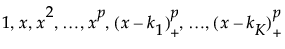
 is the positive part of (
Either a single number that designates the number of desired knot points based on percentiles of x or a vector of values that designate the internal knot points.
a = 42;
x = [1 2 3, 4 5 6, 7 8 9];
Show( Parallel Assign( {}, x[i, j] = global:a ) );
Show( x );
Parallel Assign({}, x[i,j] = global:a) = 1;
x =
[ 42 42 42,
42 42 42,
42 42 42];
Set to false (0) to use the decimal separator for your locale. Set to true (1) to always use a period (.) as a separator. The default value is false (0).
Returns a vector of indices that, used as a subscript to the original vector, sorts the vector by rank. Excludes missing values. Lists of numbers or strings are supported in addition to matrices.
Returns a vector of ranks of the values of vector, low to high as 1 to n, ties arbitrary. Lists of numbers or strings are supported in addition to matrices.
Returns a vector of ranks of the values of vector, but ranks for ties are averaged. Lists of numbers or strings are supported in addition to matrices.
Reshapes the matrix A across rows to the specified dimensions. Each value from the matrix A is placed row-by-row into the re-shaped matrix.
If ncol is not specified, the number of columns is whatever is necessary to fit all of the original values of the matrix into the reshaped matrix.
a = Matrix({ {1, 2, 3}, {4, 5, 6}, {7, 8, 9} });
[ 1 2 3,
4 5 6,
7 8 9]
Shape(a, 2);
[ 1 2 3 4 5,
6 7 8 9 1]
Shape(a, 2, 2);
[ 1 2,
3 4]
Shape(a, 4, 4);
[ 1 2 3 4,
5 6 7 8,
9 1 2 3,
4 5 6 7]
Solves a linear system. In other words, x=inverse(A)*b.
Returns a copy of a list or matrix source with the items in ascending order.
Returns a copy of a list or matrix source with the items in descending order.
x is a vector of regressor variables, y is the vector of response variables, and lambda is the smoothing argument. Larger values for lambda result in smoother splines.
Evaluates the spline predictions using the coef matrix in the same form as returned by SplineCoef(), in other words, knots||a||b||c||d. The x argument can be a scalar or a matrix of values to predict. The number of columns of coef can be any number greater than 1 and each is used for the next higher power. The powers of x are centered at the knot values. For example, the calculation for coef of knots||a||b||c||d is j is such that knots[j] is the largest knot smaller than x.
xx = x-knots[j] is the centered x value:
x is a vector of regressor variables, y is the vector of response variables, and lambda is the smoothing argument. Larger values for lambda result in smoother splines.
A‘
Vec Diag(X*Sym*X‘)