Univariate Tests and the Test for Sphericity

There are cases, such as a repeated measures model, that allow transformation of a multivariate problem into a univariate problem (Huynh and Feldt 1970). Using univariate tests in a multivariate context is valid in the following situations:

•

If the response design matrix M is orthonormal (M´M = Identity).

•

If M yields more than one response the coefficients of each transformation sum to zero.

•

If the sphericity condition is met. The sphericity condition means that the M-transformed responses are uncorrelated and have the same variance. M´ΣM is proportional to an identity matrix, where Σ is the covariance of the Y variables.

If these conditions hold, the diagonal elements of the E and H test matrices sum to make a univariate sums of squares for the denominator and numerator of an F test. Note that if the above conditions do not hold, then an error message appears. In the case of Golf Balls.jmp, an identity matrix is specified as the M-matrix. Identity matrices cannot be transformed to a full rank matrix after centralization of column vectors and orthonormalization. So the univariate request is ignored.

Example of Univariate and Sphericity Test

Select Help > Sample Data Library and open Dogs.jmp.

Select Analyze > Fit Model.

Select LogHist0, LogHist1, LogHist3, and LogHist5 and click Y.

Select drug and dep1 and click Add.

In the Construct Model Effects panel, select drug. In the Select Columns panel, select dep1. Click Cross.

For Personality, select Manova.

Click Run.

Select the check box next to Univariate Tests Also.

In the Choose Response menu, select Repeated Measures.

Time should be entered for YName, and Univariate Tests Also should be selected.

10.

Click OK.

Figure 9.8 Sphericity Test

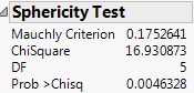
The sphericity test checks the appropriateness of an unadjusted univariate F test for the within-subject effects using the Mauchly criterion to test the sphericity assumption (Anderson 1958). The sphericity test and the univariate tests are always done using an orthonormalized M matrix. You interpret the sphericity test as follows:

•

If the true covariance structure is spherical, you can use the unadjusted univariate F-tests.

•

If the sphericity test is significant, the test suggests that the true covariance structure is not spherical. Therefore, you can use the multivariate or the adjusted univariate tests.

The univariate F statistic has an approximate F-distribution even without sphericity, but the degrees of freedom for numerator and denominator are reduced by some fraction epsilon (ε). Box (1954), Greenhouse and Geisser (1959), and Huynh-Feldt (1976) offer techniques for estimating the epsilon degrees-of-freedom adjustment. Muller and Barton (1989) recommend the Greenhouse-Geisser version, based on a study of power.

The epsilon adjusted tests in the multivariate report are labeled G-G (Greenhouse-Geisser) or H-F (Huynh-Feldt). The epsilon adjustment is shown in the value column.