Additional Example of a Logistic Plot

This example uses the Car Physical Data.jmp sample data table to show an additional example of a logistic plot. Suppose you want to use weight to predict car size (Type) for 116 cars. Car size can be one of the following, from smallest to largest: Sporty, Small, Compact, Medium, or Large.

Select Help > Sample Data Library and open Car Physical Data.jmp.

In the Columns panel, right-click on the icon to the left of Type, and select Ordinal.

Right-click on Type, and select Column Info.

From the Column Properties menu, select Value Ordering.

Verify that the data are in the following top-down order: Sporty, Small, Compact, Medium, Large.

Click OK.

Select Analyze > Fit Y by X.

Select Type and click Y, Response.

Select Weight and click X, Factor.

10.

Click OK.

The report window appears.

Figure 7.119 Example of Type by Weight Logistic Plot

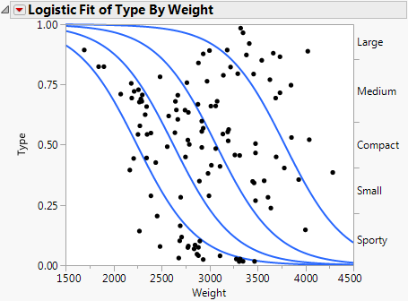
In Figure 7.119, note the following observations:

•

The first (bottom) curve represents the probability that a car at a given weight is Sporty.

•

The second curve represents the probability that a car is Small or Sporty. Looking only at the distance between the first and second curves corresponds to the probability of being Small.

•

As you might expect, heavier cars are more likely to be Large.

•

Markers for the data are drawn at their x-coordinate, with the y position jittered randomly within the range corresponding to the response category for that row.

If the x -variable has no effect on the response, then the fitted lines are horizontal and the probabilities are constant for each response across the continuous factor range. Figure 7.120 shows a logistic plot where Weight is not useful for predicting Type.

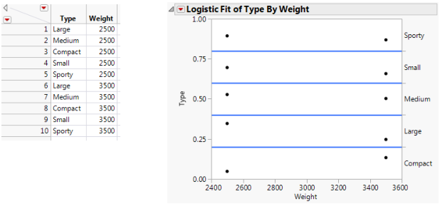
Figure 7.120 Examples of Sample Data Table and Logistic Plot Showing No y by x Relationship

Note: To re-create the plots in Figure 7.120 and Figure 7.121, you must first create the data tables shown here, and then perform steps 7-10 at the beginning of this section.

If the response is completely predicted by the value of the factor, then the logistic curves are effectively vertical. The prediction of a response is near certain (the probability is almost 1) at each of the factor levels. Figure 7.121 shows a logistic plot where Weight almost perfectly predicts Type.

Figure 7.121 Examples of Sample Data Table and Logistic Plot Showing an Almost Perfect y by x Relationship

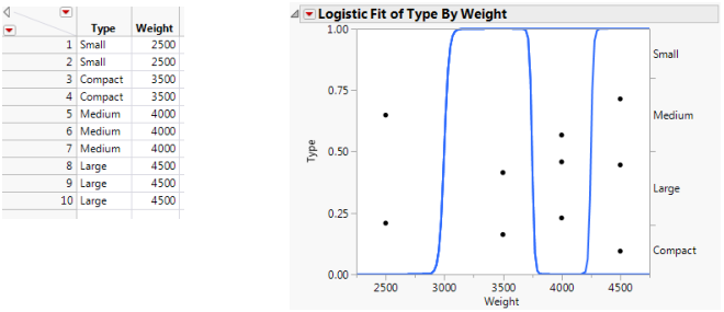
In this case, the parameter estimates become very large and are labeled unstable in the regression report. In these cases, you might consider using the Generalized Linear Model personality with Firth bias-adjusted estimates. See Launch the Generalized Linear Model Personality in the Fitting Linear Models book.