Additional Example of the Contour Profiler

Desirability functions are often used to determine the optimal settings for a response surface. The Maximize Desirability feature in the Prediction Profiler provides one combination of factor level settings that results in a predicted response that optimizes the desirability. However, there are often many factor level combinations that can optimize the desirability function. The Contour Profiler is a useful tool for finding alternative settings that optimize desirability.

This example uses the Bounce Data.jmp data table, which contains data for a tire tread experiment. The response, Stretch, is a function of three variables, Silica, Silane, and Sulfur. You will build a model and determine the optimal settings such that the value of Stretch maximizes the desirability function using the Maximize Desirability option in the Prediction Profiler. You will then use the Contour Profiler to explore other optimal settings for the specified value of Stretch.

Select Help > Sample Data Library and open Design Experiment/Bounce Data.jmp.

Click the green triangle next to the Model script, and then click Run in the launch window.

Click the Prediction Profiler red triangle menu and select Optimization and Desirability > Maximize Desirability.

Figure 3.6 Maximize Desirability Settings

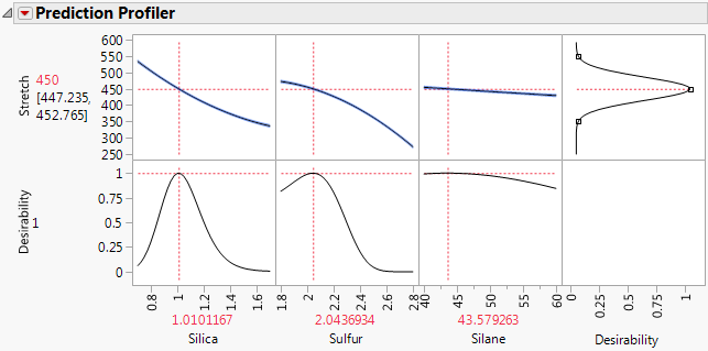
The value of Stretch that maximizes the desirability function is 450. One combination of factor level settings that results in a predicted Stretch of 450 is Silica = 1.0101, Sulfur = 2.0437, and Silane = 43.5792.

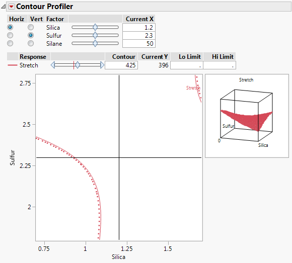
Click the red triangle menu next to Response Stretch and select Factor Profiling > Contour Profiler.

To ensure that your new setting combinations maximize desirability, you want to make sure that the settings predict Stretch within 2 units of 450. Additionally, you would like a high level of Silane, a fixed value of 60.

Figure 3.7 Contour Profiler for Bounce Data.jmp

The initial plot shows the contour values of Silica and Sulfur for Stretch at 425 and Silane at 50.

In the response controls, set the Contour value for Stretch to 450. Set the Lo Limit and High Limit for Stretch to 448 and 452, respectively. Press Enter.

Set the Current X for Silane to 60.

Figure 3.8 Contour Profiler for Optimal Settings

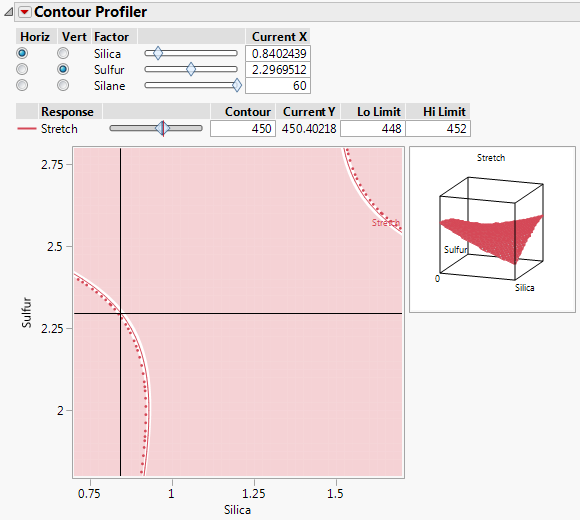
The values on the solid red curve are the Silica and Sulfur values that predict Stretch to be 450. The values within the unshaded band predict values of Stretch between 448 and 452. You can drag the crosshairs that appear on the plot to the unshaded sections to find specific settings for Silica and Sulfur. One such setting is seen in Figure 3.8.