Each of the levels of the X, Categories column defines an indicator variable. A canonical correlation is performed between the set of indicator variables representing the categories and the covariates. Linear combinations of the covariates, called canonical variables, are derived. These canonical variables attempt to summarize the between-category variation.
The first canonical variable is the linear combination of the covariates that maximizes the multiple correlation between the category indicator variables and the covariates. The second canonical variable is a linear combination uncorrelated with the first canonical variable that maximizes the multiples correlation with the categories. If the X, Categories column has k levels, then k - 1 canonical variables are obtained.
Figure 4.9 shows the Canonical Plot for a linear discriminant analysis of the data table Iris.jmp. The points have been colored by Species.
Figure 4.9 Canonical Plot for Iris.jmp
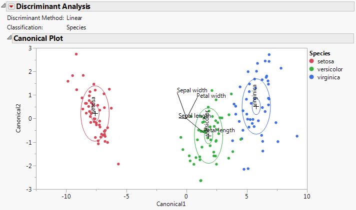
The biplot axes are the first two canonical variables. These define the two dimensions that provide maximum separation among the groups. Each canonical variable is a linear combination of the covariates. (See Canonical Structure.) The biplot shows how each observation is represented in terms of canonical variables and how each covariate contributes to the canonical variables.
|
–
|
To facilitate comparisons among the weights, the covariates are standardized so that each has mean 0 and standard deviation 1. The coefficients for the standardized covariates are called the canonical weights. The larger a covariate’s canonical weight, the greater its association with the canonical variable.
|
|
–
|
You can obtain the values of the weight coefficients by selecting Canonical Options > Show Canonical Details from the red triangle menu. At the bottom of the Canonical Details report, click Standardized Scoring Coefficients. See Standardized Scoring Coefficients for details.
|
|
•
|
Show or hide the 95% confidence ellipses by selecting Canonical Options > Show Means CL Ellipses from the red triangle menu.
|
|
•
|
Show or hide the rays by selecting Canonical Options > Show Biplot Rays from the red triangle menu.
|
|
•
|
Drag the center of the biplot rays to other places in the graph. Specify their position and scaling by selecting Canonical Options > Biplot Ray Position from the red triangle menu. The default Radius Scaling shown in the Canonical Plot is 1.5, unless an adjustment is needed to make the rays visible.
|
|
•
|
Show or hide the 50% contours by selecting Canonical Options > Show Normal 50% Contours from the red triangle menu.
|
|
•
|
Color code the points to match the ellipses by selecting Canonical Options > Color Points from the red triangle menu.
|
For the Iris.jmp data, there are three Species, so there are only two canonical variables. The plot in Figure 4.9 shows good separation of the three groups using the two canonical variables.
|
•
|
Petal length is positively associated with Canonical1 and negatively associated with Canonical2. It carries more weight in defining Canonical1 than Canonical2.
|
|
•
|
Petal width is positively associated with both Canonical1 and Canonical2. It carries about the same weight in defining both canonical variates.
|
|
•
|
Sepal width is negatively associated with Canonical1 and positively associated with Canonical2. It carries more weight in defining Canonical2 than Canonical1.
|
|
•
|
Sepal length is negatively weighted in terms of defining Canonical1 and very weakly associated in defining Canonical2.
|
Figure 4.10 shows a Canonical Plot for the sample data table Fitness.jmp. The seven continuous variates are used to classify an individual into the categories M (male) or F (female). Since the classification variable has only two categories, there is only one canonical variable.
Figure 4.10 Canonical Plot for Fitness.jmp
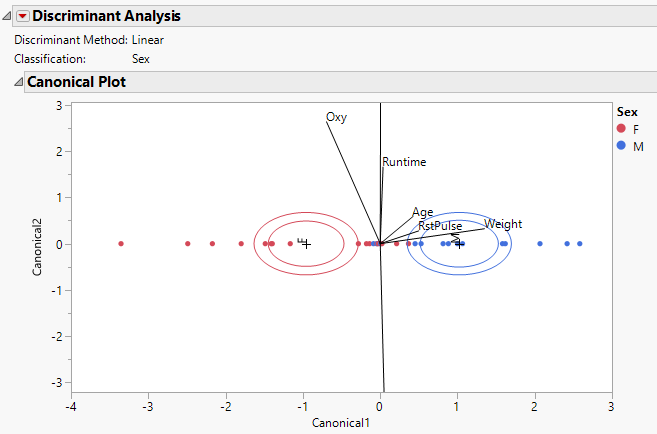
The points in Figure 4.10 have been colored by Sex. Note that the two groups are well separated by their values on Canonical1.
|
•
|
|
•
|
Weight, RstPulse, and Age are positively associated with Canonical1. Weight has the highest degree of association. The covariates RstPulse and Age have a similar, but smaller, degree of association.
|
|
•
|
Oxy is negatively associated with Canonical1.
|