 Construct Nonparametric Confidence Intervals for Variance Components
In this example, you are interested in the effects of temperature, time, and the amount of catalyst on a reaction. Temperature is a very-hard-to-change variable (whole plot factor), time is hard-to-change (subplot factor), and the amount of catalyst is easy-to-change. For information on whole plot and subplot factors, see Numbers of Whole Plots and Subplots in the Design of Experiments Guide.
|
•
|
 Construct the Design
If you prefer to skip the steps in this section, select Help > Sample Data Library and open Design Experiment/Catalyst Design.jmp. In the Catalyst Design.jmp data table, click the green triangle next to the DOE Simulate script. Then go to Fit the Model.
|
1.
|
Select DOE > Custom Design.
|
|
2.
|
In the Factors outline, type 3 next to Add N Factors.
|
|
3.
|
Click Add Factor > Continuous.
|
|
4.
|
|
5.
|
This defines Temperature to be a whole plot factor.
|
6.
|
This defines Time to be a subplot factor.
|
7.
|
Click Continue.
|
|
8.
|
In the Model outline, select Interactions > 2nd.
|
|
9.
|
Click the Custom Design red triangle and select Simulate Responses.
|
Note: Setting the Random Seed in step 10 and Number of Starts in step 11 reproduces the exact results shown in this example. In constructing a design on your own, these steps are not necessary.
|
10.
|
(Optional) Click the Custom Design red triangle and select Set Random Seed. Type 12345 and click OK.
|
|
11.
|
(Optional) Click the Custom Design red triangle and select Number of Starts. Type 1000 and click OK.
|
|
12.
|
Click Make Design.
|
|
13.
|
Click Make Table.
|
Note: The entries in your Y and Y Simulated columns will differ from those that appear in Figure 9.151.
Figure 9.151 Design Table
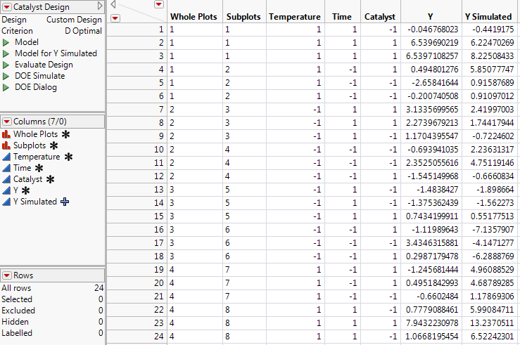
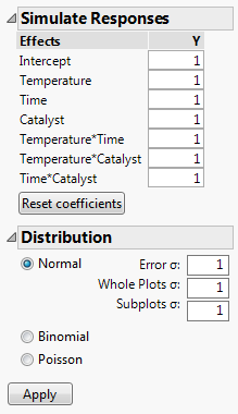
Figure 9.152 Simulate Responses Window
The design table and a Simulate Responses window appear. Notice that the design table contains a DOE Simulate script. At any time, you can run this script to specify different parameter values.
 Fit the Model
|
1.
|
|
2.
|
|
3.
|
Click Apply.
|
In the data table, the formula for Y Simulated updates to reflect your specifications. To view the formula, click on the plus sign to the right of the column name in the Columns panel.
|
4.
|
In the data table, click the green triangle next to the Model script.
|
|
5.
|
|
6.
|
This action replaces Y with a column that contains a simulation formula.
|
7.
|
Click Run.
|
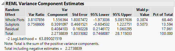
Note: Because the values in Y Simulated are randomly generated, the entries in your report will differ from those that appear in Figure 9.153.
Figure 9.153 REML Report Showing Wald Confidence Intervals
 Generate Confidence Intervals
|
1.
|
In the REML Variance Components Estimates outline, right-click in the Var Component column and select Simulate.
|
Figure 9.154 Simulate Window
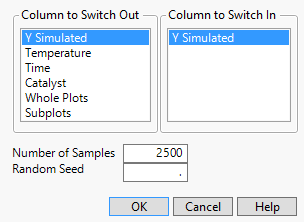
In your simulations, you replace the column Y Simulated, which you used to run your model, with a new instance of the column Y Simulated, which generates a new column of simulated values for each simulation. The column on which you right-clicked and that appears as selected, Var Component, will be simulated for each effect listed in the Parameter Estimates table.
|
2.
|
|
3.
|
(Optional) Next to Random Seed, enter 456.
|
This reproduces the values shown in Figure 9.155, except for the values in row 1.
|
4.
|
Click OK.
|
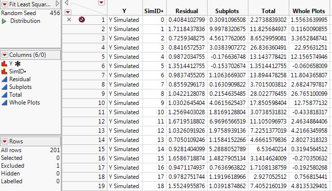
The first row of the Fit Least Squares Simulate Results (Var Component) data table contains the initial values of Var Component and is excluded. The remaining rows contain simulated values.
|
5.
|
Run the Distribution script.
|
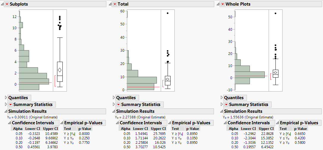
For each variance component, confidence intervals at various confidence levels are shown in the Simulation Results report (Figure 9.156). Compare the 95% intervals in the Alpha=0.05 row of each table to the intervals given in the REML report (Figure 9.153):