Shows plots of least squares means for nominal and ordinal effects. If the effect is an interaction, this option displays the Least Squares Means Plot Options window. See LSMeans Plot.
Shows the Contrast Specification window, which enables you to specify and test contrasts to compare levels for nominal and ordinal effects and their interactions. See LSMeans Contrast.
Shows tests and confidence intervals for pairwise comparisons of least squares means using Student’s t tests. See LSMeans Student’s t and LSMeans Tukey HSD.
Note: The significance level applies to individual comparisons and not to all comparisons collectively. The error rate for the collection of comparisons is greater than the error rate for individual tests.
Shows tests and confidence intervals for pairwise comparisons of least squares means using the Tukey-Kramer HSD (Honestly Significant Difference) test (Tukey 1953; Kramer 1956). See LSMeans Student’s t and LSMeans Tukey HSD.
Note: The significance level applies to the collection of pairwise comparisons. The significance level is exact if the sample sizes are equal and conservative if the sample sizes differ (Hayter 1984).
Shows tests and confidence intervals for pairwise comparisons against a control level that you specify. Also provides a plot of test results. See LSMeans Dunnett.
For each level of each column in the interaction, jointly tests pairwise comparisons among all the levels of the other classification columns in the interaction. See Test Slices.
Shows the Power Details report, which enables you to analyze the power for the effect test. For details, see Power Analysis.
Least squares means are values predicted by the model for the levels of a categorical effect where the other model factors are set to neutral values. The neutral value for a continuous effect is defined to be its sample mean. The neutral value for a nominal effect that is not involved in the effect of interest is the average of the coefficients for that effect. The neutral value for an uninvolved ordinal effect is defined to be the first level of the effect in the value ordering.
Least squares means are also called adjusted means or population marginal means. Least squares means can differ from simple means when there are other effects in the model. In fact, it is common for the least squares means to be closer together than the sample means. This situation occurs because of the nature of the neutral values where these predictions are made.
Because least squares means are predictions at specific values of the other model factors, you can compare them. When effects are tested, comparisons are made using the least squares means. For further details about least squares means, see Least Squares Means across Nominal Factors in Statistical Details and Ordinal Least Squares Means.
|
1.
|
|
2.
|
Select Analyze > Fit Model.
|
|
3.
|
|
4.
|
|
5.
|
|
6.
|
Click Run.
|
The Effect Details report, shown in Figure 2.10, shows reports for each of the three effects. Least Squares Means tables are given for age and sex, but not for the continuous effect height. Notice how the least squares means differ from the sample means.
Figure 2.10 Least Squares Mean Table
The LSMeans Plot option produces a Least Squares Means Plot for nominal and ordinal main effects and their interactions. If the effect is an interaction, this option displays the Least Squares Means Plot Options window. See Least Squares Means Plot Options.
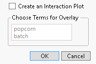
Figure 2.11 Least Squares Means Plot Options Window
To create the report in Figure 2.12, follow these steps:
|
1.
|
|
2.
|
Select Analyze > Fit Model.
|
|
3.
|
|
4.
|
Select popcorn, oil amt, and batch and click Macros > Full Factorial. Note that the Emphasis changes to Effect Screening.
|
|
5.
|
Click Run.
|
|
7.
|
|
8.
|
Select LSMeans Plot from the popcorn*batch red triangle menu. The Least Squares Means Plot Options window appears.
|
|
9.
|
|
10.
|
|
11.
|
Click OK.
|
|
12.
|
|
13.
|
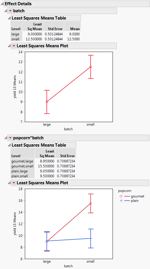
Figure 2.13 shows the popcorn*batch interaction plot with the factors transposed. Compare it with the plot in Figure 2.12. These plots depict the same information but, depending on your interest, one might be more intuitive than the other.
A contrast is a linear combination of parameter values. In the Contrast Specification window, you can specify multiple contrasts and jointly test whether they are zero (Figure 2.14).
Each time you click the + or - button, the contrast coefficients are normalized to make their sum zero and their absolute sum equal to two, if possible. To compare additional levels, click the New Column button. A new column appears in which you define a new contrast. After you are finished, click Done. The Contrast report appears (Figure 2.15). The overall test is a joint F test for all contrasts.
p-value for the significance test
The Test Detail report (Figure 2.15) shows a column for each contrast that you tested. For each contrast, the report gives its estimated value, its standard error, a t ratio for a test of that single contrast, the corresponding p-value, and its sum of squares.
The Parameter Function report (Figure 2.15) shows the contrasts that you specified expressed as linear combinations of the terms of the model.
|
1.
|
|
2.
|
Select Analyze > Fit Model.
|
|
3.
|
|
4.
|
|
5.
|
Select age in the Select Columns list, select height in the Construct Model Effects list, and click Cross.
|
|
6.
|
Click Run.
|
|
7.
|
Figure 2.14 LSMeans Contrast Specification for age
|
10.
|
Note that there is a text box next to the continuous effect height. The default value is the mean of the continuous effect.
|
|
11.
|
Click Done.
|
The Contrast report is shown in Figure 2.15. The test for the contrast is significant at the 0.05 level. You conclude that the predicted weight for age 12 and 13 children differs statistically from the predicted weight for age 14 and 15 children at the mean height of 62.55.
Figure 2.15 LSMeans Contrast Report
The LSMeans Student’s t and LSMeans Tukey HSD (honestly significant difference) options test pairwise comparisons of model effects.
|
•
|
The LSMeans Student’s t option is based on the usual independent samples, equal variance t test. Each comparison is based on the specified significance level. The overall error rate resulting from conducting multiple comparisons exceeds that specified significance level.
|
Figure 2.16 shows the LSMeans Tukey report for the effect age in the Big Class.jmp sample data table. (You can obtain this report by running the Fit Model data table script and selecting LS Means Tukey HSD from the red triangle menu for age.) By default, the report shows the Crosstab Report and the Connecting Letters Report.
Figure 2.16 LSMeans Tukey HSD Report
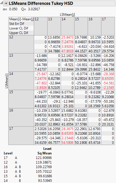
In Figure 2.16, levels 17, 12, 16, 13, and 15 are connected by the letter A. The connection indicates that these levels do not differ at the 0.05 significance level. Also, levels 16, 13, 15, and 14 are connected by the letter B, indicating that they do not differ statistically. However, ages 17 and 14, and ages 12 and 14, are not connected by a common letter, indicating that these two pairs of levels are statistically different.
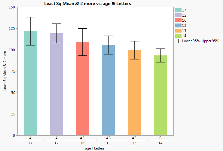
Figure 2.17 shows the bar chart for an example based on Big Class.jmp. Run the Fit Model data table script, select LSMeans Tukey HSD from the red triangle menu for age. Select Save Connecting Letters Table from the LSMeans Differences Tukey HSD report. Run the Bar Chart script in the data table that appears.
Ranks the differences from largest to smallest, giving standard errors, confidence limits, and p-values. Also plots the differences on a bar chart with overlaid confidence intervals.
Gives individual detailed reports for each comparison. For a given comparison, the report shows the estimated difference, standard error, confidence interval, t ratio, degrees of freedom, and p-values for one- and two-sided tests. Also shown is a plot of the t distribution, which illustrates the significance test for the comparison. The area of the shaded portion is the p-value for a two-sided test.
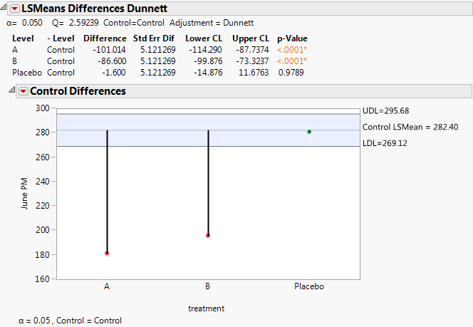
Dunnett’s test (Dunnett 1955) compares a set of means against the mean of a control group. The error rate applies to the collection of pairwise comparisons. The LSMeans Dunnett option conducts Dunnett’s test for the levels of the given effect. Hsu’s factor analytical approximation is used for the calculation of p-values and confidence intervals (Hsu 1992).
A report for the LSMeans Dunnett option for effect treatment in the Cholesterol.jmp sample data table is shown in Figure 2.18. Here, the response is June PM and the level of treatment called Control is specified as the control level.
Figure 2.18 LSMeans Dunnett Report
The Test Slice reports follow the same format as do the LSMeans Contrast reports. See LSMeans Contrast.
Opens the Power Details window, where you can enter information to obtain retrospective or prospective details for the F test of a specific effect.
Note: To ensure that your study includes sufficiently many observations to detect the required differences, use information about power when you design your experiment. Such an analysis is called a prospective power analysis. Consider using the DOE platform to design your study. Both DOE > Sample Size and Power and DOE > Evaluate Design are useful for prospective power analysis. For an example of a prospective power analysis using standard least squares, see Prospective Power Analysis.
Figure 2.19 shows an example of the Power Details window for the Big Class.jmp sample data table. Using the Power Details window, you can explore power for values of alpha (α), sigma (σ), delta (δ), and Number (study size). Enter a single value (From only), two values (From and To), or the start (From), stop (To), and increment (By) for a sequence of values. Power calculations are reported for all possible combinations of the values that you specify.
Figure 2.19 Power Details Window
Alpha (α)
Sigma (σ)
Delta (δ)
The effect size of interest. See Effect Size for details. The initial value, shown in the first row, is the square root of the sum of squares for the hypothesis divided by the square root of the number of observations in the study; that is,  .
.
.Number (n)
Solves for the power as a function of α, σ, δ, and n. The power is the probability of detecting a difference of size δ by seeing a test result that is significant at level α, for the specified σ and n. For more details, see Computations for the Power in Statistical Details.
Solves for the smallest number of observations required to obtain a test result that is significant at level α, for the specified δ and σ. For more details, see Computations for the LSN in Statistical Details.
Solves for the smallest positive value of a parameter or linear function of the parameters that produces a p-value of α. The least significant value is a function of α, σ, and n. This option is available only for one-degree-of-freedom tests. For more details, see Computations for the LSV in Statistical Details.
Retrospective power calculations use estimates of the standard error and the test parameters in estimating the F distribution’s noncentrality parameter. Adjusted power is retrospective power calculation based on an estimate of the noncentrality parameter from which positive bias has been removed (Wright and O’Brien 1988).
The adjusted power deals with a sample estimate, so it and its confidence limits are computed only for the δ estimated in the current study. For more details, see Computations for the Adjusted Power in Statistical Details.