|
1.
|
In the JMP Home Window, select File > New > Script. This opens a new script window.
|
dt = New Table( "Sales Model" );
dt << New Column( "Unit Sales", Values( {1000, 2000} ) );
dt << New Column( "Unit Price", Values( {2, 4} ) );
dt << New Column( "Unit Cost", Values( {2, 2.5} ) );
dt << New Column( "Revenue",
Formula( :Unit Sales * :Unit Price )
);
dt << New Column( "Total Cost",
Formula( :Unit Sales * :Unit Cost + 1200 )
);
dt << New Column( "Profit",
Formula( :Revenue - :Total Cost ),
Set Property( "Spec Limits", {LSL( 0 )} )
);
Profiler(
Y( :Revenue, :Total Cost, :Profit ),
Objective Formula( Profit )
);
 to run the script. Alternatively, you can select Ctrl-R.
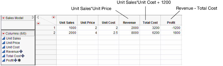
The script creates the data table in Figure 7.24 with some initial scaling data and stores formulas into the output variables. It also launches the Prediction Profiler.
Figure 7.24 Data Table Created from Script
|
5.
|
|
–
|
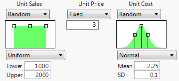
Unit Sales is Uniform with Lower limit 1000 and Upper limit 2000.
|
|
–
|
Unit Price is Fixed at 3.
|
|
–
|
Unit Cost is Normal with mean of 2.25 and standard deviation of 0.1.
|
Figure 7.25 Specifications for Prediction Profiler
|
7.
|
Click the Simulate button.
|
Note: Your numbers might differ from those shown in Figure 7.26 due to the random draws in the simulation.
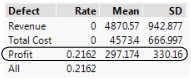
Figure 7.26 Simulator
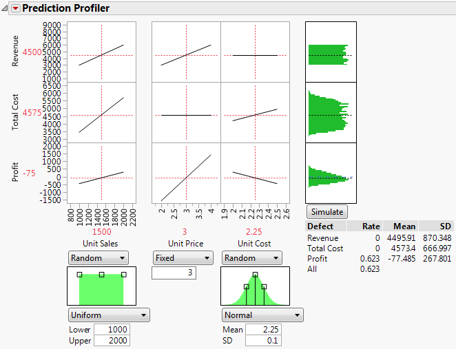
It appears that the models are unlikely to be profitable. By putting a lower specification limit of zero on Profit, the defect report tells you that the probability of being unprofitable is 62%.
|
8.
|
Change the fixed value of Unit Price to 3.25.
|
|
9.
|
Click the Simulate button.
|
Figure 7.27 Results