To demonstrate a possible workflow with the Defect Profiler, we use Tiretread.jmp. The experimental data in the Tiretread.jmp sample data table comes from an experiment to study the effects of SILICA, SILANE, and SULFUR on four measures of tire tread performance.
|
1.
|
|
2.
|
Select Graph > Profiler.
|
|
3.
|
Select Pred Formula ABRASION, Pred Formula MODULUS, Pred Formula ELONG, and Pred Formula HARDNESS and click Y, Prediction Formula.
|
|
4.
|
Click OK.
|
|
5.
|
|
6.
|
Click the Simulator red triangle and select Spec Limits.
|
|
8.
|
Click Save to save the Spec Limits to the data table.
|
|
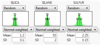
9.
|
Beneath each factor, select Random.
|
Figure 7.9 Profiler Random Specifications
|
1.
|
Click the Simulator red triangle and select Defect Profiler.
|
Figure 7.10 Defect Profiler
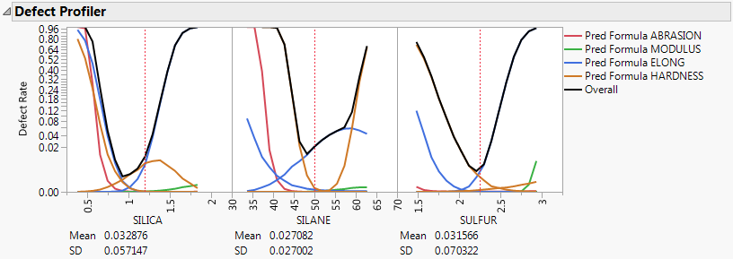
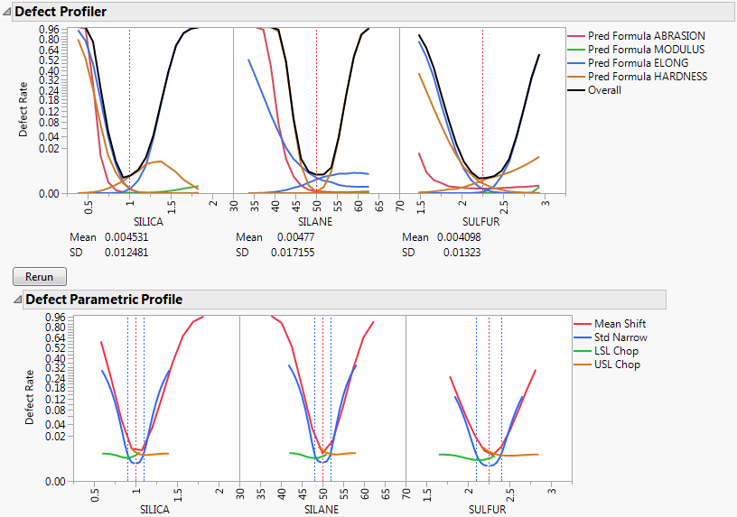
Note: The defect profiler is based on simulation with random inputs. The values that you obtain might differ from those shown in Figure 7.10.
Consider the overall curve for SILICA. As silica varies, the defect rate goes from the lowest rate of 0.001 when silica is about 1 and increases quickly up to a defect rate of nearly 1 as silica increases or decreases from 1. However, SILICA is itself random. If you integrate the density curve of SILICA, you would estimate the average defect rate to be about 0.03, which is shown as the Mean for SILICA. This estimate of the overall defect rate estimated by the simulation is shown in the defect table under the simulation histograms. The Mean value for the overall defect rate for all factors are similar.
The Defect Profiler also includes an estimate of the standard deviation of the defect rate with respect to the variation in each factor. This value (labeled SD) is 0.057 for SILICA. The standard deviation is related to the sensitivity of the defect rate with respect to the distribution of that factor. Comparing the SD values across the three factors, the SD for SULFUR is higher than the SD values for SILICA and SILANE. This indicates that to improve the defect rate, shifting the distribution in SULFUR should have the greatest effect. A distribution can be shifted by changing its mean, changing its standard deviation, or by truncating the distribution by rejecting inputs that do not meet certain specification limits.
|
2.
|
Click the Simulator red triangle and select Defect Parametric Profile.
|
Figure 7.11 Defect Parametric Profile
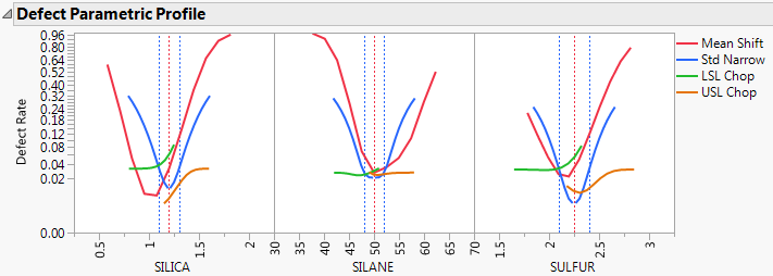
Consider SULFUR and note that the current defect rate (0.03) is represented in four ways corresponding to each of the four curves in the Parametric Profiler.
For the red curve, Mean Shift, the current rate is where the red curve intersects the vertical red dotted line. The Mean Shift curve represents the change in overall defect rate as the mean of SULFUR changes. One opportunity to reduce the defect rate is to shift the mean slightly to the left. If you use the crosshair tool on this plot, you see that a shift down in the mean reduces the defect rate to about 0.02.
For the blue curve, Std Narrow, the current defect rate is where the blue curve intersects the two dotted blue lines. The Std Narrow curves represent the change in defect rate as the standard deviation changes. The dotted blue lines represent one standard deviation below and above the current mean. The blue curve is drawn symmetrically around the center. At the center, the blue curve reaches a minimum, representing the defect rate for a standard deviation of zero. That is, if we totally eliminate variation in SULFUR, the defect rate is about 0.003. This is much lower than the current rate of 0.03. If you look at the other defect parametric profile curves, you can see that this is better than reducing variation in the other factors, something that we suspected by the SD value for SULFUR.
For the green curve, LSL Chop, there are no interesting opportunities for improvement in the defect rate. The green curve is above current defect rates for the entire range of the curve. This indicates that reducing the variation by rejecting parts with too-small values for SULFUR does not help reduce the defect rate.
The orange curve, USL Chop, suggests a way to improve the defect rate. Reading the curve from the right, the curve starts out at the current defect rate (0.03). Then as you start rejecting more parts by decreasing the USL for SULFUR, the defect rate improves. However, moving a spec limit to the center of the distribution is equivalent to throwing away half the parts, which might not be a practical solution.
Looking at all the opportunities over all factors, it now looks like there are two good options for further investigation. You could shift the mean of SILICA to about 1 or reduce the variation in SULFUR. Because it is generally easier in practice to change a process mean than a process variation, the best first adjustment might be to shift the mean of SILICA to 1.
|
3.
|
In the Prediction Profiler, adjust the Mean of SILICA from 1.2 to 1.0.
|
|
4.
|
The Defect Profiler updates based on the adjusted SILICA value.
Figure 7.12 Adjusted Defect Rates