Launch the Mixed Model Personality

Mixed Model is one of several personalities that you can select in the Fit Model launch window. This section describes how you select Mixed Model as your fitting methodology in the Fit Model launch window. Options that are specific to this selection are also covered.

Fit Model Launch Window

You can specify models with fixed effects, random effects, a repeated structure or a combination of those. The options differ based on the nature of the model that you specify.

To fit models using the mixed model personality, select Analyze > Fit Model and then select Mixed Model from the Personality list. Note that when you enter a continuous variable in the Y list before selecting a Personality, the Personality defaults to Standard Least Squares.

When fitting models using the Mixed Model personality, you can allow unbounded variance components. This means that variance components that have negative estimates are not reported as zero. This option is selected by default. It should remain selected if you are interested in fixed effects, because bounding the variance estimates at zero leads to bias in the tests for fixed effects. See Negative Variances in Standard Least Squares Report and Options for more information about the Unbounded Variance Components option.

Fixed Effects Tab

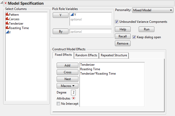
Add all fixed effects on the Fixed Effects tab. Use the Add, Cross, Nest, Macros, and Attributes options as needed. For more information about these options, see the Model Specification topic.

The fixed effects for analysis of the Split Plot.jmp sample data table appear in Figure 7.7. Note that it is possible to have no fixed effects in the model. For an example, see Spatial Example: Uniformity Trial.

Figure 7.7 Fit Model Launch Window Showing Completed Fixed Effects

Random Effects Tab

Specify traditional variance component models and random coefficients models using the Random Effects tab.

Variance Components

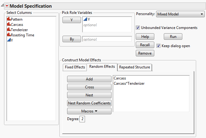
For a traditional variance component model, specify terms such as random blocks, whole plot error terms, and subplot error terms using the Add, Cross, or Nest options. For more information about these options, see the Model Specification topic.

Figure 7.8 shows the random effects specification for the Split Plot.jmp sample data where Carcass is a random block. Split Plot Example describes the example in detail.

Figure 7.8 Fit Model Launch Window Showing Completed Random Effects Tab

Random Coefficients

To construct random coefficients models, use the Nest Random Coefficients button to create groups of random coefficients.

Select the continuous columns from the Select Columns list that are predictors.

Select the Random Effects tab and then Add.

Select these effects in the Random Effects tab. Also select the column that contains the random effect whose levels define the individual regression models. This column is essentially the subject in a random statement in SAS PROC MIXED.

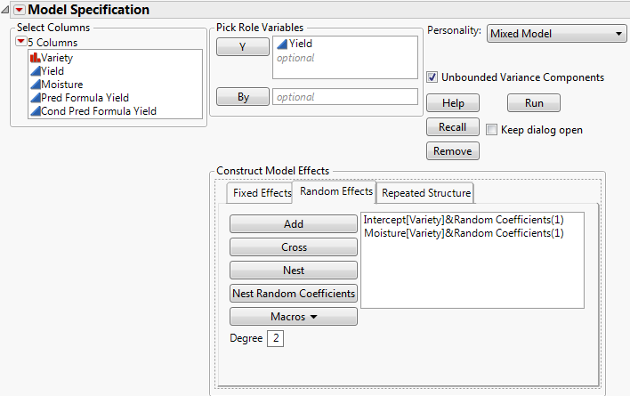
Click the Nest Random Coefficients button.

This last step creates random intercept and random slope effects that are correlated within the levels of the random effect. The subject is nested within the other effects due to the variability among subjects. If you believed that the intercept might be fixed for all groups, you would select Intercept[<group>]&Random Coefficients(1) and then click Remove.

You can define multiple groups of random coefficients in this fashion, as in hierarchical linear models. This might be necessary when you have both a random batch effect and a random batch by treatment effect on the slope and intercept coefficients. This might also be necessary in a hierarchical linear model: when you have a random student effect and random school effect on achievement scores and students are nested within school.

Random coefficients are modeled using an unstructured covariance structure. Figure 7.9 shows the random coefficients specification for the Wheat.jmp sample data. (See also Example Using Mixed Model.)

Figure 7.9 Completed Fit Model Launch Window Showing Random Coefficients

Repeated Structure Tab

Use the Repeated Structure tab to select a covariance structure for repeated effects in the model.

Figure 7.10 Completed Fit Model Launch Window Showing Repeated Structure Tab

Structure

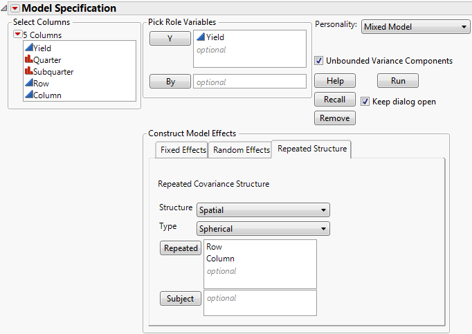
The repeated structure is set to Residual by default. The Residual structure specifies that there is no covariance between observations, namely, the errors are independent. All other covariance structures model covariance between observations. For more information about the structures, see Repeated Measures and Antedependent Covariance Structure in the Statistical Details section.

Table 7.1 lists the covariance structures available, the requirements for using each structure, and the number of covariance parameters for the given structure. The number of observation times is denoted by J.

Table 7.1 Repeated Covariance Structure Requirements
Structure	Repeated Column Type	Required Number of Repeated Columns	Subject	Number of Parameters
Residual	not applicable	0	not applicable	0
Unequal Variances	categorical	1	optional	J
Unstructured	categorical	1	required	J(J+1)/2
AR(1)	continuous	1	optional	2
Compound Symmetry	categorical	1	required	2
Antedependent Equal Variance	categorical		required	J
Toeplitz	categorical	1	required	J
Compound Symmetry Unequal Variances	categorical	1	required	J+1
Antedependent	categorical		required	2J-1
Toeplitz Unequal Variances	categorical	1	required	2J-1
Spatial	continuous	2+	optional
Spatial Anisotropic	continuous	2+	optional
Spatial with Nugget	continuous	2+	optional
Spatial Anisotropic with Nugget	continuous	2+	optional

If you enter a Repeated or Subject column with the Residual structure, those columns are ignored. This alert appears: “Repeated columns and subject columns are ignored when the Residual covariance structure is selected.”

Type

When you select one of the spatial covariance structures, a Type list appears from which you select a type of spatial structure. Four Types are available: Power, Exponential, Gaussian, and Spherical. Figure 7.10 shows the Spatial Spherical selection for the Uniformity Trial.jmp sample data.

Repeated

Enter columns that define the repeated measures structure. The modeling types of Repeated columns depend on the covariance structure. See Table 7.1 for more information.

Subject

Enter one or more columns that define the Subject. Subject columns must be categorical.