Launch the Principal Components Platform

Launch the Principal Components platform by selecting Analyze > Multivariate Methods > Principal Components. Principal Component analysis is also available using the Multivariate and the Scatterplot 3D platforms.

The example described in Example of Principal Component Analysis uses all of the continuous variables from the Solubility.jmp sample data table.

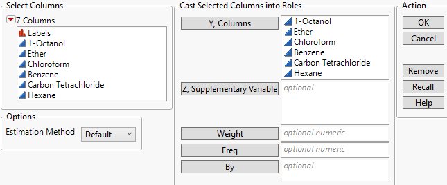
Figure 3.3 Principal Components Launch Window

Y, Columns

The variables to analyze for components.

Z, Supplementary Variable

The supplementary variables to be displayed. Supplementary variables are not included in the calculation of principal components and including them does not affect the results. Supplementary variables that are continuous can be projected on to the loading plot and used to enhance interpretation.

Weight

Identifies one column whose numeric values assign a weight to each row in the analysis.

Note: The Weight role is ignored for the Wide and Sparse estimation methods.

Freq

Identifies one column whose numeric values assign a frequency to each row in the analysis.

Note: The Freq role is ignored for the Wide and Sparse estimation methods.

Creates a Principal Component report for each value specified by the By column so that you can perform separate analyses for each group.

Estimation Method

Specifies the method for calculating the correlations. Several of these methods address the treatment of missing data.

Default

The Default option uses either the Row-wise, Pairwise, or REML methods. A JMP Alert also recommends switching to the Wide method when appropriate.

–

Row-wise estimation is used for data tables with no missing values.

–

Pairwise estimation is used for data tables with missing values and either more than 10 columns, more than 5,000 rows, or more columns than rows.

–

REML estimation is used otherwise.

–

Wide estimation is recommended by a JMP Alert window for data tables with more than 500 columns. This is because computation time can be considerable when you use the other methods with a large number of columns. Click Wide to switch to the Wide method or click Continue to use the method you originally selected.

REML

Restricted maximum likelihood (REML) estimation uses all of the data, even if missing values are present. Due to a bias-correction factor, this method is slow if the dataset is large and there are many missing values. Therefore, REML is most useful for smaller datasets. If there are no missing cells in the data, then the REML and ML estimates are equivalent and equal to the sample covariance matrix. If there are missing cells, REML’s variance and covariance estimates are less biased than the estimates from ML estimation. For more information, see REML.

Maximum likelihood (ML) estimation uses all of the data, even if missing values are present. Because the estimates from ML are generated quickly, this method is most useful for large data tables with missing data.

Robust

Robust estimation uses all of the data, even if missing values are present. This method down-weights extreme values and is therefore useful for data tables that might have outliers. For statistical details, see Robust in Correlations and Multivariate Techniques.

Row-wise

Row-wise estimation does not use observations with missing values, so rows that contain missing cells are deleted before the method is applied. This method is useful for excluding any observations that have missing data. Row-wise estimation was the only estimation method available prior to JMP 8, so it can also be used to check compatibility with JMP versions prior to JMP 8.

Pair-wise

Pair-wise estimation uses all of the data, even if missing values are present. This estimation method performs correlations for all rows for each pair of columns with nonmissing values. It is most useful when a data table has missing values and either more columns than rows, more than 10 columns, or more than 5,000 rows.

Wide

Wide estimation does not use observations with missing values, so rows that contain missing cells are deleted before the method is applied. This estimation method uses an algorithm based on the full singular value decomposition. The algorithm avoids calculating the covariance matrix and is therefore computationally efficient. It is useful when you have a very large number of columns in your data. For additional information, see Wide.

Sparse