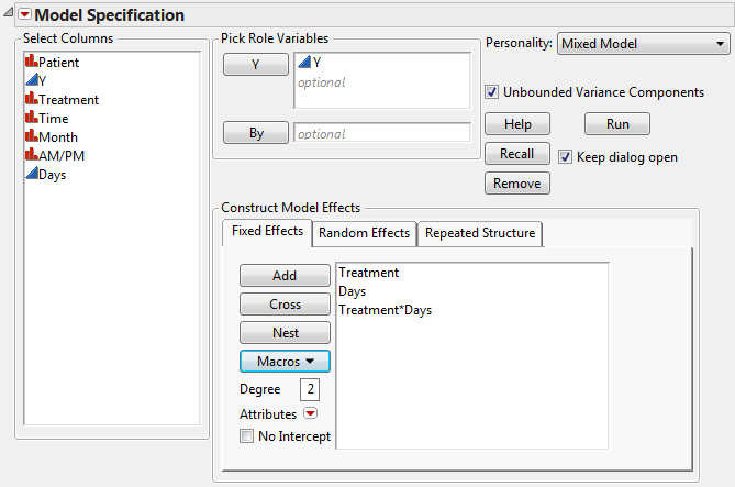
Consider the Cholesterol Stacked.jmp sample data table. A study was performed to test two new cholesterol drugs against a control drug. Five patients with high cholesterol were randomly assigned to each of four treatments (the two experimental drugs, the control, and a placebo). Each patient’s total cholesterol was measured at six times during the study: the first day in April, May, and June in the morning and afternoon. You are interested in whether either of the new drugs is effective at lowering cholesterol and in whether time and treatment interact.
Suppose that your model has J observation times. Then the number of covariance parameters in the covariance matrices for the three structures available are as follows:
|
•
|
|
•
|
See Repeated Measures for more information.
Open Cholesterol.jmp to see a format that is typically used for recording repeated measures data. For Mixed Model analysis of this data, each cholesterol measurement needs to be in its own row, as in Cholesterol Stacked.jmp. To construct Cholesterol Stacked.jmp, the data in Cholesterol.jmp was stacked using Tables > Stack.
The Days column in the stacked table was constructed using a formula. The Days column gives the number days into the study when the cholesterol measurement was taken. Its modeling type is continuous. This is necessary because the AR(1) covariance structure requires the repeated effect be continuous.
|
1.
|
|
2.
|
Select Analyze > Fit Model.
|
|
3.
|
Select Keep dialog open so that you can return to the launch window in the next example.
|
|
4.
|
|
5.
|
Select Mixed Model from the Personality list.
|
|
6.
|
|
7.
|
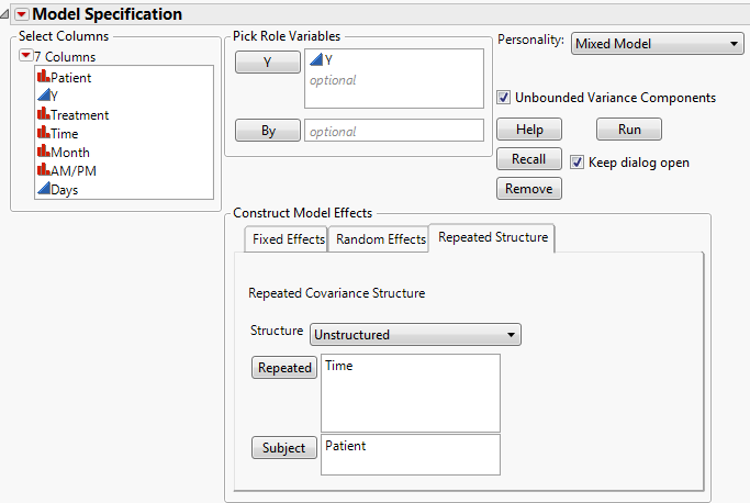
Select the Repeated Structure tab.
|
|
8.
|
Select Unstructured from the Structure list.
|
|
9.
|
|
10.
|
|
11.
|
Click Run.
|
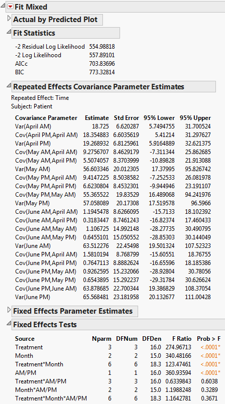
The Fit Mixed report is shown in Fit Mixed Report - Unstructured Covariance Structure. Because you want to compare your three models using AICc or BIC, you are interested in the Fit Statistics report. The AICc for the unstructured model is 703.84.
|
1.
|
|
2.
|
|
3.
|
If you are continuing from the previous example, remove Time and Patient. Otherwise, a warning appears: “Repeated columns and subject columns are ignored when the Residual covariance structure is selected.” You are given the option to click OK to continue the analysis.
|
|
4.
|
Select the Random Effects tab.
|
|
5.
|
|
6.
|
|
7.
|
Click Run.
|
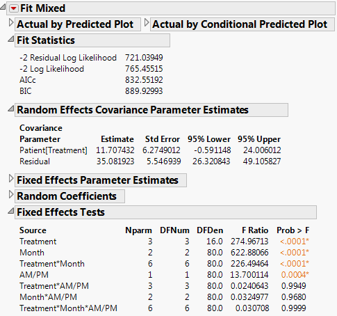
The Fit Mixed report is shown in Fit Mixed Report - Residual Error Covariance Structure. The Fit Statistics report shows that the AICc for the Residual model is 832.55, as compared to 703.84 for the Unstructured model.
|
1.
|
|
2.
|
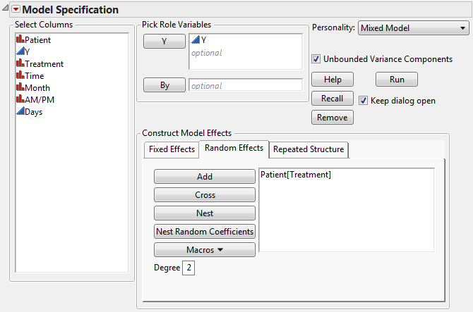
If you are continuing from the previous example, select Patient[Treatment] on the Random Effects tab and then click Remove.
|
|
3.
|
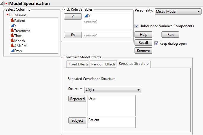
Select the Repeated Structure tab.
|
|
4.
|
Select AR(1) from the Structure list.
|
|
5.
|
|
6.
|
|
7.
|
Click Run.
|
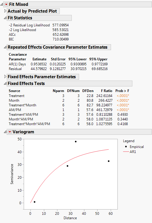
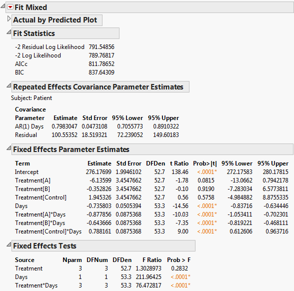
The Fit Mixed report is shown in Fit Mixed Report - AR(1) Covariance Structure. The Fit Statistics report shows that the AICc for the AR(1) model is 652.63, compared with 832.55 for the Residual model and 703.84 for the Unstructured model. Based on the AICc criterion, the AR(1) model is the best of the three models.
The AR(1) structure requires the estimation of two covariance parameters. These estimates are shown in the Repeated Effects Covariance Parameter Estimates report. The AR(1) Days parameter estimate is an estimate of ρ, the correlation parameter in the AR(1) structure.
The Variogram plot shows the empirical semivariances and the curve for the AR(1) model. Since there are only five non-zero values for Days, only four distance classes are possible and only four points are shown. The AR(1) structure seems appropriate. To explore other structures, select options from the red triangle menu next to Variogram.
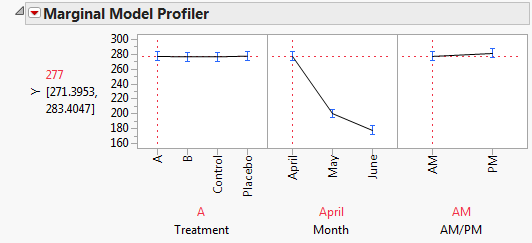
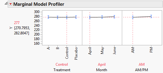
To explore these significant effects, select Marginal Model Inference > Profiler from the Fit Mixed report’s red triangle menu. The Marginal Model Profiler report (Marginal Profiler Plot for Treatment A) shows that, for Treatments A and B, cholesterol levels (Y) decrease steadily over the three months. However, when you set Treatment to Control or Placebo, you see virtually no change over the three months (Marginal Profiler Plot for Control).
Note that Treatment A seems to result in lower cholesterol readings in May than Treatment B does. If this effect is significant, it might indicate that Treatment A acts more quickly than B. The next section, Compare All Treatments in June, shows you how to evaluate the treatments.
The profiler also shows the main effect of AM/PM. To obtain the profiler, select Marginal Model Inference > Profiler. By setting Treatment and Month to all 12 combinations of their levels, you see that the predicted cholesterol level is consistently higher in the afternoon than in the morning.
|
2.
|
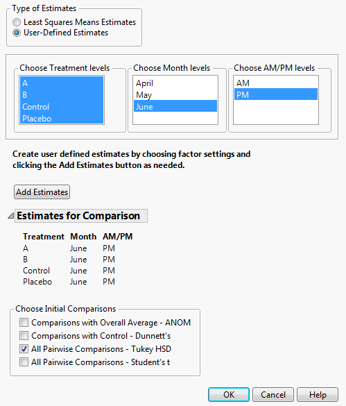
Under Types of Estimates, select User-Defined Estimates.
|
|
6.
|
Click Add Estimates.
|
|
7.
|
From the Choose Initial Comparisons list, select All Pairwise Comparisons - Tukey HSD.
|
|
8.
|
Click OK.
|
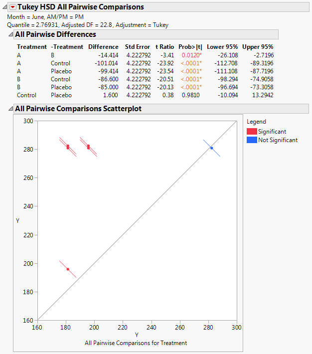
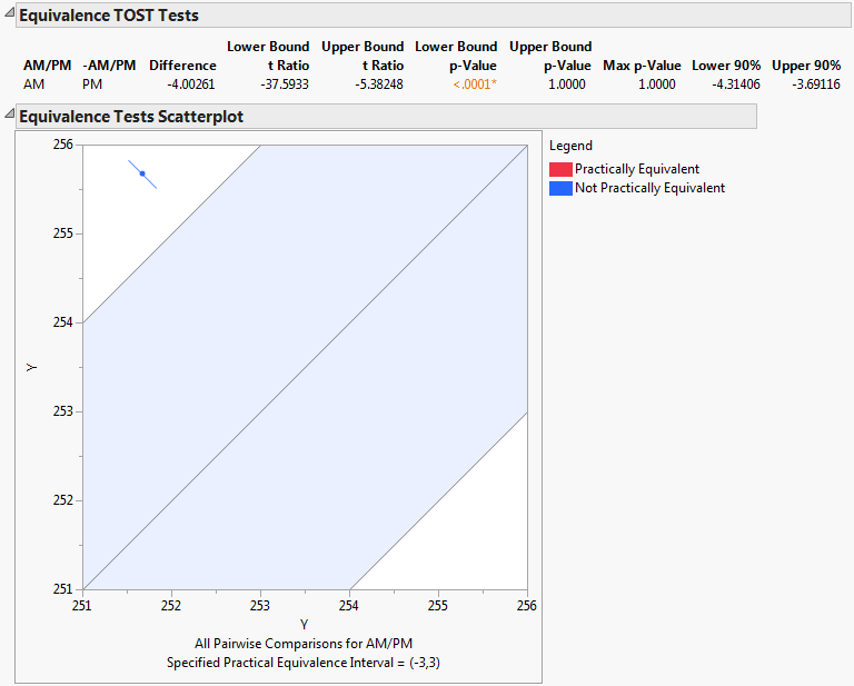
The Tukey HSD All Pairwise Comparisons report shows an All Pairwise Differences report and an All Pairwise Comparisons Scatterplot (Tukey HSD All Pairwise Comparisons Report for All Treatments for June PM). All treatments other than the Control and Placebo differ significantly on the June PM measurements.
|
1.
|
Select Multiple Comparisons from the Fit Mixed red triangle menu.
|
|
2.
|
Select AM/PM from the Choose an Effect list.
|
|
3.
|
Select All Pairwise Comparisons - Tukey HSD from the Choose Initial Comparisons list.
|
|
4.
|
Click OK.
|
|
5.
|
Select Equivalence Tests from the Tukey HSD All Pairwise Comparisons red triangle menu.
|
|
6.
|
Type 3 in the box for Difference considered practically zero.
|
|
7.
|
Click OK.
|
|
1.
|
After following steps in Covariance Structure: AR(1) Example, return to the Fit Model launch window.
|
|
3.
|
|
4.
|
Click Run.
|
The Fit Mixed report is shown in Fit Mixed Report - AR(1) Covariance Structure with Continuous Fixed Effect. You see that the interaction of Treatment and Days is highly significant indicating different regressions for the drugs.
Note: To predict outcomes for the drugs at different days, use the profiler. See the Profilers book for more information.
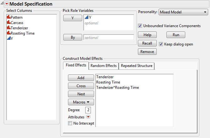
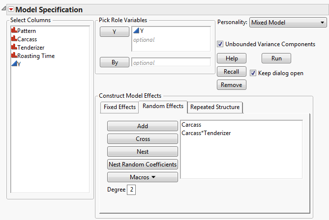
The data in the Split Plot.jmp sample data table come from a study of the effects of tenderizer and length of cooking time on meat. Six beef carcasses were randomly selected from carcasses at a meat packaging plant. From the right rib-eye muscle of each carcass, three rolled roasts were prepared under uniform conditions. Each of these three roasts was assigned a tenderizing treatment at random. After treatment, a coring device was used to mark four cores of meat near the center of each.
|
1.
|
|
2.
|
Select Analyze > Fit Model.
|
|
3.
|
|
4.
|
Select Mixed Model from the Personality list.
|
|
5.
|
|
6.
|
Select the Random Effects tab.
|
|
7.
|
|
8.
|
|
9.
|
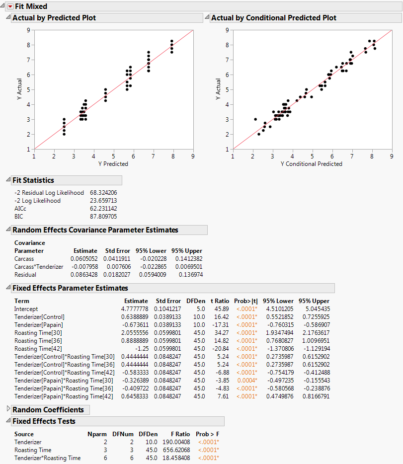
Click Run.
|
|
1.
|
Select Marginal Model Inference > Profiler from the Fit Mixed report’s red triangle menu.
|
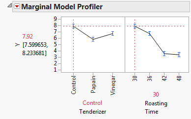
In Marginal Model Profiler with Roasting Time Set to 30 Minutes, notice that both the papain and vinegar tenderizers result in significantly lower tenderness scores than the control when roasting time is either 30 or 36 minutes. However, at 42 minutes, there are no significant differences. At 48 minutes, papain gives a value lower than the control, but vinegar does not. Papain gives lower tenderness scores than does vinegar at all times except 42 minutes.
|
3.
|
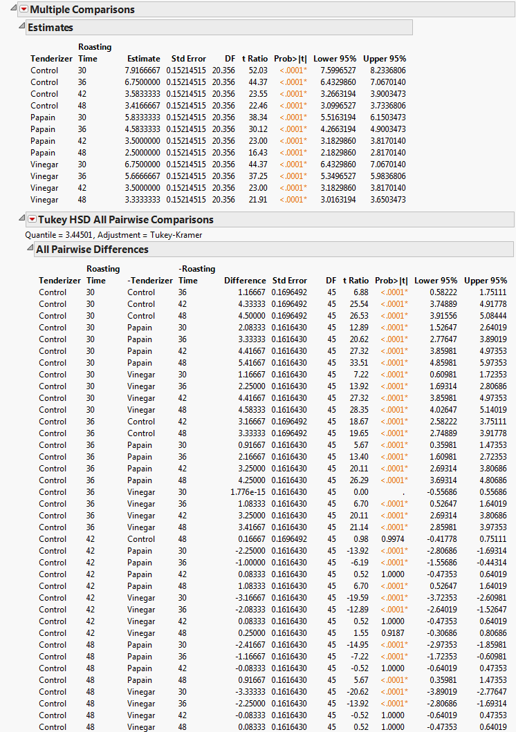
Select Multiple Comparisons from the Fit Mixed red triangle menu.
|
|
4.
|
Select Tenderizer*Roasting Time.
|
|
5.
|
Multiple Comparisons, Partial View shows a partial list of pairwise comparisons. Most of the differences between papain and vinegar that you observed in the profiler are statistically significant. Therefore, it appears that papain is the better tenderizer.
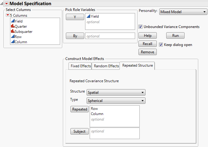
Consider the Uniformity Trial.jmp sample data table. An agronomic uniformity trial was conducted on an 8x8 grid of plots. In a uniformity trial, a test crop is grown on a field with no experimental treatments applied. The response variable, often yield, is measured. The idea is to characterize variability in the field as background for planning a designed experiment to be conducted on that field. (See SAS for Mixed Models, 2nd Edition, 2006, pp. 447.)
Once you have established whether there is a nugget effect, you determine the best fitting spatial covariance structure. Finally, you fit the blocking models and compare these to the best spatial structure. In this example, both AICc and BIC are used to select a best model. Spatial and Temporal Variability provides more information about nugget effects and other spatial terminology.
To determine whether there is significant spatial variability, you can fit a model that accounts for spatial variability. Then you can compare the likelihood for this spatial model to the likelihood for a model that does not account for spatial variability. You can do this because the independent errors model is nested within the spatial model family: The independent errors model is a spatial model with spatial correlation, ρ, equal to 0. This means that you can perform a formal likelihood ratio test of the two models.
|
1.
|
|
2.
|
Select Analyze > Fit Model.
|
|
3.
|
Select Keep dialog open so that you can return to the launch window in the next example.
|
|
4.
|
|
5.
|
Select Mixed Model from the Personality list.
|
|
6.
|
Select the Repeated Structure tab.
|
|
7.
|
Choose Spatial from the list next to Structure.
|
|
8.
|
Choose Spherical from the list next to Type.
|
|
9.
|
|
10.
|
Click Run.
|
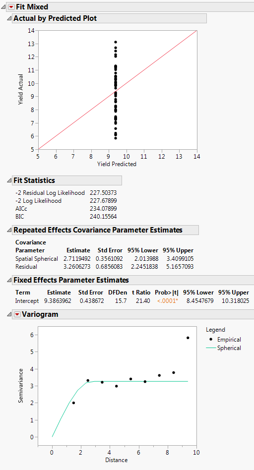
The Fit Mixed report is shown in Fit Mixed Report - Spatial Spherical. The Actual by Predicted Plot shows that the predicted yield is a single value. This is because only spatial covariance was fit. The Fit Statistics report shows that -2 Log Likelihood is 227.68, and the AICc is 234.08.
Because an isotropic spatial structure was fit, a Variogram plot is shown. Because the trials are laid out in an 8 by 8 grid, there will be more pairs of points at small distances than at very large distances. See Graph Builder Plot of Proposed Complete and Incomplete Block Designs for the layout. The Variogram shows that a spherical spatial structure is an excellent fit for distances up to about 8.4. The distance class for the final distance consists of only the two diagonal pairs of points.
The Repeated Effects Covariance Parameter Estimates report gives estimates of the range (Spatial Spherical = 2.71) and the sill (Residual = 3.26). See Variogram.
|
2.
|
Select Repeated Structure tab.
|
|
3.
|
Select Residual from the Structure list.
|
|
4.
|
Remove Row and Column from the Repeated effects list. Otherwise, a warning appears: “Repeated columns and subject columns are ignored when the Residual covariance structure is selected.”
|
|
5.
|
Click Run.
|
You can conduct a likelihood ratio test in this example, because the independent errors model is nested within the spatial model family. The independent errors model is a spatial model with spatial correlation, ρ, equal to 0. This means that you can perform a formal likelihood ratio test of the two models.
In this example, the likelihood ratio test statistic is 254.22-227.68=26.54. Comparing this to a Chi-square distribution on one degree of freedom, the null hypothesis of no spatial correlation is rejected with a p-value < 0.0001. You can conclude that these data contain significant spatial variability.
|
2.
|
Select the Repeated Structure tab.
|
|
3.
|
|
4.
|
Select Spatial with Nugget from the Structure list.
|
|
5.
|
Select Spherical from the Type list.
|
|
6.
|
Click Run.
|
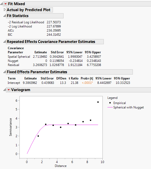
The Fit Mixed report is shown in Fit Mixed Report - Spatial Spherical with Nugget. Notice that the log likelihoods are essentially equal to those of the spherical with no nugget model, and the AICc is slightly higher (236.36 compared to 234.08). The Repeated Effects Covariance Parameter Estimates report shows that the Nugget covariance parameter has an estimate of zero. There does not appear to be any evidence for a nugget effect.
|
7.
|
From the red triangle menu next to Variogram, select Spatial > Spherical.
|
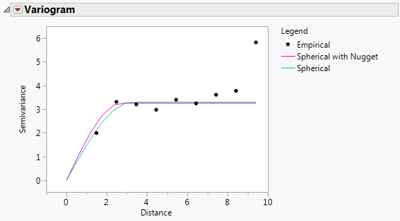
The Variogram report is shown in Fit Mixed Report - Variogram. The two variograms are virtually identical. This also suggests that there is no evidence of a nugget effect.
|
9.
|
Select Repeated Structure tab.
|
|
10.
|
To test anisotropicity, select Spatial Anisotropic from the Structure list.
|
|
11.
|
Select Spherical from the Type list.
|
|
12.
|
Click Run.
|
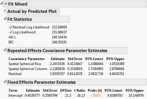
The Fit Mixed report is shown in Fit Mixed Report - Spatial Anisotropic Spherical. The fit statistics indicate not as good a fit as the isotropic (spatial structure) spherical model (AICc 240.54 compared to 234.08). The Repeated Effects Covariance Parameter Estimates report shows that the estimates for the Row (Spatial Spherical Row) and Column (Spatial Spherical Column) covariances are very close. There is no evidence to suggest that spatial correlations within rows and columns of the grid differ.
Repeat step 1 through step 4 in Select the Type of Spatial Covariance. Change Spatial with Nugget to Spatial and then change Spherical to the other available types: Power, Exponential, Gaussian. The observed AICc values for these types and the other fits that you performed are summarized in Fit Statistics for Spatial Models Fit.
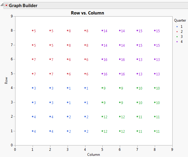
Run the Graph Builder script from the Uniformity Trial.jmp sample data table. Graph Builder Plot of Proposed Complete and Incomplete Block Designs shows the plot of the proposed complete and incomplete block designs for the field. The color indicates the quarter fields that would serve as complete blocks. The numbered points represent the subquarter fields that would serve as incomplete blocks.
|
2.
|
Select Repeated Structure tab.
|
|
3.
|
Select Residual from the Structure list.
|
|
4.
|
Remove Row and Col from the effect. Otherwise, a pop-up dialog appears, stating, “Repeated columns and subject columns are ignored when the Residual covariance structure is selected.”
|
|
5.
|
Select the Random Effects tab.
|
|
6.
|
|
7.
|
Click Run.
|
|
8.
|
Both AICc’s and BICs for the competing models are shown in Fit Statistics for Spatial and Block Models. The spherical covariance structure results in the best model fit. This indicates that, for future studies using this field, a completely randomized design with spatially correlated errors is preferred.
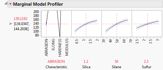
Consider the Tiretread Stacked.jmp sample data table. The effect of three factors (Silica, Silane, and Sulfur) is studied for four responses (Abrasion, Modulus, Elong, and Hardness).
Open Tiretread.jmp to see a format that is typically used for recording repeated measures data. For Mixed Model analysis of this data, each repeated measurement needs to be in its own row, as in Tiretread Stacked.jmp. To construct Tiretread Stacked.jmp, the data in Tiretread.jmp was stacked using Tables > Stack.
|
1.
|
|
2.
|
Select Analyze > Fit Model.
|
|
3.
|
|
4.
|
Select Mixed Model from the Personality list.
|
|
5.
|
|
6.
|
|
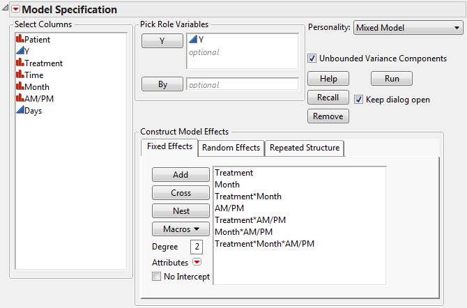
8.
|
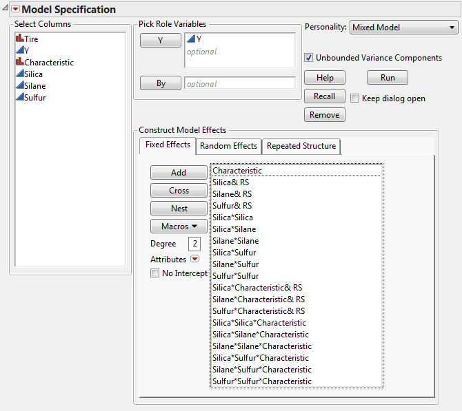
Select Characteristic from the Select Columns list.
|
|
9.
|
Click Cross.
|
Fit Model Launch Window Showing Completed Fixed Effects Tab shows the completed fixed effects tab.
|
10.
|
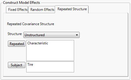
Select the Repeated Structure tab.
|
|
11.
|
Select Unstructured from the Structure list.
|
|
12.
|
|
13.
|
|
14.
|
Click Run.
|
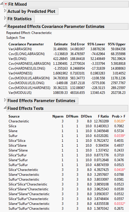
The Fit Mixed report is shown in Fit Mixed Report. The Repeated Effects Covariance Parameter Estimates report gives the estimated variances and covariances for the four responses. All of the confidence intervals for the covariance estimates include zero. This suggests that the analysis of the responses that treats them as independent is not necessarily incorrect. Although, there might not be enough data to detect nonzero covariances.
The Fixed Effects Test report indicates that Characteristic is significant. This is expected. However, note that the Silane*Sulfur*Characteristic and Silica*Characteristic interactions are significant. The significance of the Silane*Sulfur*Characteristic reflects the fact that, for the usual univariate analysis, Silane*Sulfur is significant for some responses and not for others. Although Silica is significant for all responses, the significance of the Silica*Characteristic interaction suggests that Silica impacts the four responses differently.
|
1.
|
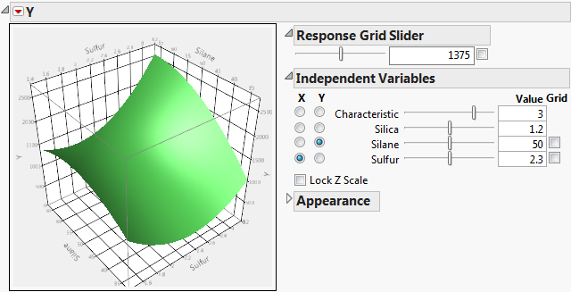
Select Marginal Model Inference > Surface Profiler from the Fit Mixed red triangle menu.
|
|
2.
|
|
3.
|
Note that Surface Profiler Showing the Response Surface for MODULUS and Silica = 1.2 shows a cross-section of the response surface for the Silica value 1.2.
|
1.
|
Select Marginal Model Inference > Profiler from the Fit Mixed red triangle menu.
|
The predicted values shown in the profiler match those obtained using the univariate analysis. However, the model includes effects that involve Characteristic. This makes it easier for you to identify the impact of the operational factors. Profiler for the Correlated Tire Tread Analysis shows the profiler for ABRASION. The Y scale is changed to display the effects of Silica, Silane, and Sulfur more effectively.