The Liver Cancer.jmp sample data table contains liver cancer Node Count values for 136 patients. It also includes measurements on six potentially related variables: BMI, Age, Time, Markers, Hepatitis, and Jaundice. These columns are described in Column Notes in the data table.
This example develops a prediction model for Node Count using the six predictors. Node Count is modeled using a Poisson distribution.
|
1.
|
|
2.
|
Select Analyze > Fit Model.
|
|
3.
|
|
4.
|
This adds all terms up to degree 2 (the default in the Degree box) to the model.
|
5.
|
|
6.
|
From the Personality list, select Generalized Regression.
|
|
7.
|
From the Distribution list, select Poisson.
|
|
8.
|
Click Run.
|
|
9.
|
Click Go.
|
|
10.
|
From the report’s red triangle menu, select Select Nonzero Terms.
|
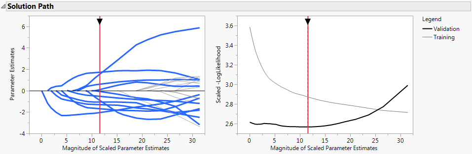
The Solution Path is shown in Solution Path for Lasso Fit with Nonzero Terms Highlighted. The paths for terms that have nonzero coefficients are highlighted. Think of the solution paths as moving from right to left across the plot, as the solutions shrink farther from the MLE. A number of terms have paths that shrink them to zero fairly early.
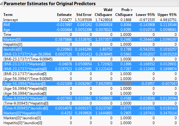
The Parameter Estimates for Original Predictors report (Parameter Estimates Report with Nonzero Terms Highlighted) shows the parameter estimates for the centered and scaled data. The Parameter Estimates for Original Predictors report shows the estimates for the uncentered and unscaled data. The 11 terms with nonzero parameter estimates are highlighted in both reports. These include interaction effects. In the data table, all six predictor columns are selected because every predictor column appears in a term that has a nonzero coefficient.
In the Effect Tests report, the 10 effects with zero coefficient estimates are designated as Removed. The Effect Tests report indicates that only one effect is significant at the 0.05 level: the Age*Markers interaction.
|
11.
|
Click on the row for (Age - 56.3994)*Markers[0] in either the Parameter Estimates for Original Predictors or the Parameter Estimates for Centered and Scaled Predictors report.
|
This action highlights that effect’s path in the Solution Path plot and selects the columns Age and Markers in the data table.
|
12.
|
From the Adaptive Lasso with Validation Column Validation report’s red triangle menu, select Save Columns > Save Prediction Formula and Save Columns > Save Variance Formula.
|
|
13.
|
Right-click either column heading and select Formula to view the formula. Alternatively, click on the plus sign to the right of the column name in the Columns panel.
|
The prediction formula in the Save Prediction Formula column applies the exponential function to the estimated linear part of the model. The prediction variance formula in Node Count Variance is given by the identical formula, because the variance of a Poisson distribution equals its mean.
This example shows how to develop a prediction model for the binomial response, Severity, in the Liver Cancer.jmp sample data table.
|
1.
|
|
2.
|
Select Analyze > Fit Model.
|
|
3.
|
|
4.
|
All terms up to degree 2 (the default in the Degree box) are added to the model.
|
5.
|
|
6.
|
From the Personality list, select Generalized Regression.
|
|
7.
|
From the Distribution list, select Binomial.
|
|
8.
|
Click Run.
|
|
9.
|
Select Elastic Net as the Estimation Method.
|
|
10.
|
Click Go.
|
The Effect Tests report also shows that there are no significant terms at the 0.05 level. However, the Time*Markers interaction has a small p-value of 0.0650 and the Time effect has a small p-value of 0.1512.
|
12.
|
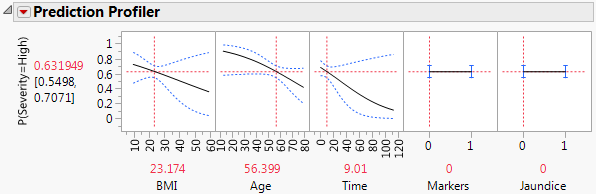
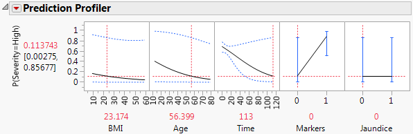
To see how Time and the Time*Markers interaction affect Severity, select Profiler from the Adaptive Elastic Net report’s red triangle menu.
|
|
13.
|
Move the red dashed line for Time from left to right to see its interaction with Markers (Profiler for Probability That Severity = High, Time Low and Profiler for Probability That Severity = High, Time High). For patients who enter the study with small values of Time since diagnosis, Markers have little impact on Severity. But for patients who enter the study having been diagnosed for a longer time, Markers are important. For those patients, normal markers suggest a lower probability of high Severity.
|
The Fishing.jmp sample data table contains fictional data for a study of various factors that affect the number of fish caught by groups visiting a park. The data table contains 250 responses from families or groups of traveling companions. This example models the number of Fish Caught as a function of Live Bait, Fishing Poles, Camper, People, and Children. These columns are described in Column Notes in the data table.
The data table contains a hidden column called Fished. During data collection, it was never determined whether anyone in the group had actually fished. However, the Fished column is included in the table to emphasize the point that catching zero fish can happen in one of two ways: Either no one in the group fished, or everyone who fished in the group was unlucky.
|
1.
|
|
2.
|
Select Analyze > Fit Model.
|
|
3.
|
|
4.
|
Terms up to degree 2 (the default in the Degree box) are added to the model.
|
5.
|
|
6.
|
From the Personality list, select Generalized Regression.
|
|
7.
|
From the Distribution list, select ZI Poisson.
|
|
8.
|
Click Run.
|
|
9.
|
From the Estimation Method List, select Elastic Net.
|
|
10.
|
Click Go.
|
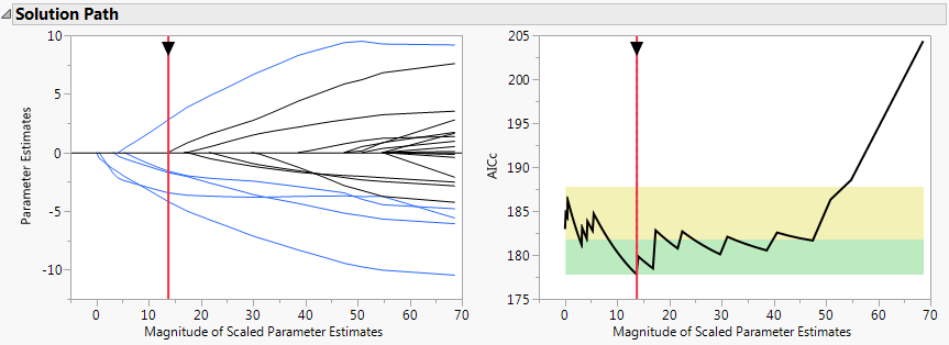
The Solution Path, both Parameter Estimates reports, and the Effect Tests report indicate that a fair number of terms are zeroed. The Zero Inflation parameter, whose estimate is shown on the last line of both Parameter Estimates reports, is highly significant. This indicates that some of the variation in the response, Fish Caught, might be due to the fact that some groups did not fish.
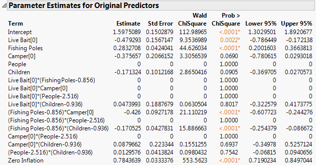
The Effect Tests report indicates that four terms are significant at the 0.05 level: Live Bait, Fishing Poles, Fishing Poles*Camper, and Fishing Poles*Children.
|
11.
|
Select Profiler from the red triangle menu for the Adaptive Elastic Net with Validation Column Validation report.
|
|
12.
|
From the Profiler report’s red triangle menu, select Desirability Functions.
|
A function is imposed on the response, which indicates that maximizing the number of Fish Caught is desirable. (See the Profilers book for more information about desirability functions.)
|
13.
|
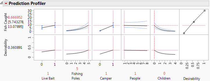
From the Profiler report’s red triangle menu, select Maximize Desirability.
|
The Profiler, with settings that maximize the number of fish caught, is shown in Prediction Profiler with Fish Caught Maximized. You can vary the settings to see the impact of the significant effects: Live Bait, Fishing Poles, Fishing Poles*Camper, and Fishing Poles*Children. For example, live bait is associated with more fish; campers tend to bring more fishing poles than those not camping and therefore catch more fish.
|
14.
|
From the Adaptive Elastic Net with Validation Column Validation report’s red triangle menu, select Save Columns > Save Prediction Formula and Save Columns > Save Variance Formula.
|
|
15.
|
Right-click either column heading and select Formula to view the formula. Alternatively, click the plus sign to the right of the column name in the Columns panel. Note the appearance of the estimated zero-inflation parameter, 0.7843639, in both of these formulas.
|