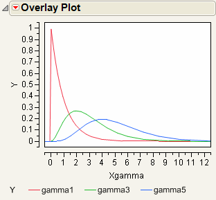
Overlay Plot normally assumes you want a function plot when the Y column contains a formula. However, formulas that contain random number functions are more frequently used with simulations, where function plotting is not often wanted. Therefore, the Function Plot option is off by default when a random number function is present, but on for all other functions.
|
1.
|
|
2.
|
|
3.
|
|
4.
|
|
5.
|
Click OK.
|
|
6.
|
A second y-axis is useful for plotting data with different scales on the same plot, such as a stock’s closing price and its daily volume, or temperature and pressure. For example, consider plotting the selling price of an inexpensive stock against the Dow Jones Industrial Average.
|
1.
|
|
2.
|
|
3.
|
|
4.
|
|
5.
|
|
6.
|
Click OK.
|
|
7.
|
From the red triangle menu for Overlay Plot, select Y Options > Connect Points.
|
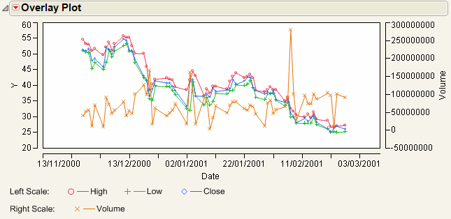
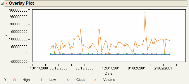
The variables High, Low, and Close are the stock prices of the same stock and thus are on the same scale. Volume is a different scale entirely, representing the trading volume of the entire Dow Jones Industrial Average.
To see why this matters, perform the same steps above without clicking the Left Scale/Right Scale button for Volume. Compare the resulting graph in Single Axis Overlay Plot to Dual Axis Overlay Plot.
|
1.
|
|
2.
|
|
3.
|
|
4.
|
|
5.
|
Click OK.
|
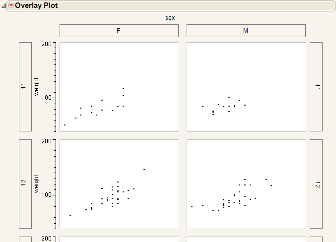
Select the Separate Axes option from the red triangle menu to produce plots that do not share axes. Compare Grouped Plots Without Separate Axes to Grouping Variables.