Creates a data table containing a row for each response with a column called Response Name that identifies the responses. Four additional columns contain the Lower Limit, Upper Limit, Response Goal, and Importance. Saving responses allows you to quickly load them into a DOE window.
Note: It is possible to create a factors table by typing data into an empty table, but remember to assign each column an appropriate Design Role. Do this by right-clicking on the column name in the data grid and selecting Column Properties > Design Role. In the Design Role area, select the appropriate role.
The constraint table contains a column for each linear constraint. The first rows contain the coefficients for each factor. The last row contains the inequality bound. Each constraint’s column contains a column property called ConstraintState that identifies the constraint as a “less than” or a “greater than” constraint. See Column Properties in Column Properties.
Note: You can set a preference to always simulate responses. Select File > Preferences > Platforms > DOE. Check Simulate Responses.
Saves scripts called Moments Matrix and Model Matrix to the design data table. These scripts contain the moments and design matrices. Use these in scripts that you write. See Save X Matrix.
Changes the design optimality criterion. The default criterion, Recommended, specifies D-optimality for all design types, unless you added quadratic effects using the RSM button in the Model outline. For more information about the D-, I-, and alias-optimal designs, see Optimality Criteria.
Note: You can set a preference to always use a given optimality criterion. Select File > Preferences > Platforms > DOE. Check Optimality Criterion and select your preferred criterion.
Enables you to specify the number of random starts used in constructing the design. See Number of Starts.
Maximum number of seconds spent searching for a design. The default search time is based on the complexity of the design. See Design Search Time and Number of Starts.
If the iterations of the algorithm require more than a few seconds, a Computing Design progress window appears. If you click Cancel in the progress window, the calculation stops and gives the best design found at that point. The progress window also displays D-efficiency for D-optimal designs that do not include factors with Changes set to Hard or Very Hard or with Estimability set to If Possible.
Note: You can set a preference for Design Search Time. Select File > Preferences > Platforms > DOE. Check Design Search Time and enter the maximum number of seconds. In certain situations where more time is required, JMP extends the search time.
Constrains the continuous factors in a design to a hypersphere. Specify the radius and click OK. Design points are chosen so that their distance from 0 equals the Sphere Radius. Select this option before you click Make Design.
Bayesian D- or I-optimality is used in constructing designs with If Possible factors. The default values used in the algorithm are 0 for Necessary terms, 4 for interactions involving If Possible terms, and 1 for If Possible terms. For more details, see The Alias Matrix in Technical Details and Optimality Criteria.
For the definition of D-efficiency, see Optimality Criteria. For details about alias optimality, see Alias Optimality.
Specify the difference in the mean response that you want to detect for model effects. See Set Delta for Power.
Note: You can set a preference to always save the matrix script. Select File > Preferences > Platforms > DOE. Check Save X Matrix.
The model matrix describes the design for the experiment. The model matrix has a row for each run and a column for each term of the model specified in the Model outline. For each run, the corresponding row of the model matrix contains the coded values of the model terms.
Continuous terms are coded to range from -1 to 1. Nominal terms are coded by applying the Gram-Schmidt orthogonalization procedure to JMP’s coding for nominal effects. Find additional information about coding for nominal effects in the Fitting Linear Models book. See also The Model Matrix in Technical Details.
The moments matrix is dependent upon the model effects but is independent of the design. It is defined as follows:
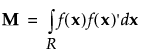
where  denotes the model effects corresponding to factor combinations of the vector of factors,
  , and R denotes the design space. For additional details concerning moments and design matrices, see Goos and Jones (2011, pp 88-90) and Myers et al. (2009). Note that the moments matrix is called a matrix of region moments in Myers et al. (2009, p. 376).
From the Custom Design red triangle menu, select Save X Matrix. After the design and the table are created, in the Custom Design table, the Moments Matrix and Model Matrix scripts, and if the design is a split plot, the V Inverse script, are saved as table properties.
|
•
|
Select Edit from the red triangle next to either the Moments Matrix, Model Matrix, or V Inverse script. The script shows the corresponding matrix. You can copy this matrix into scripts that you write.
|
|
1.
|
|
2.
|
Add 3 continuous factors and click Continue.
|
|
3.
|
Click Interactions > 2nd.
|
|
4.
|
From the Custom Design red triangle menu, select Save X Matrix.
|
|
5.
|
|
6.
|
In the Table panel, select Edit from the red triangle next to Moments Matrix.
|
The script appears in a script window. The script shows the moments matrix, which is called Moments.
|
7.
|
|
8.
|
In the Table panel, select Run Script from the red triangle next to Moments Matrix.
|
The number of rows appear in the log as N Row(Moments)=7.
|
9.
|
In the Table panel, select Edit from the red triangle next to Model Matrix.
|
|
10.
|
Select Run Script from the red triangle next to Model Matrix.
|
The number of rows appears in the log as N Row(X)=12.
|
12.
|
Select Run Script.
|
The number of starts is the number of times that the coordinate-exchange algorithm initiates with a new design. See Coordinate-Exchange Algorithm. You can specify your own value using the Number of Starts option. Increasing the number of random starts tends to improve the optimality of the resulting design.
Design Search Time is the amount of time allocated to finding an optimal design. Custom Design’s coordinate-exchange algorithm consists of finding near-optimal designs based on random starting designs. See Coordinate-Exchange Algorithm. The Design Search Time determines how many designs are constructed based on random starting designs.
You can specify your own value using the Design Search Time option. Increasing the search time tends to improve the optimality of the resulting design.
By default, delta is set to 2. The default coefficient for each continuous effect is set to 1. An n-level categorical factor is represented by n–1 indicator variables. The default coefficients for the n–1 terms (which represent the categorical factor) are alternating values of 1 and -1. The default coefficients for an interaction effect with more than one degree of freedom are also alternating values of 1 and -1.