Defect Profiler Example

To show a common workflow with the Defect profiler, we use Tiretread.jmp. The experimental data in the Tiretread.jmp sample data table results from an experiment to study the effects of SILICA, SILANE, and SULFUR on four measures of tire tread performance.

1.	Select Help > Sample Data Library and open Tiretread.jmp.

2.	Select Graph > Profiler.

3.	From the Prediction Profiler’s red triangle menu, select Simulator.

4.	Select Spec Limits from the Simulator red triangle menu.

5.	For each response, enter the spec limits as shown in Spec Limits. Click Save.

6.	For each factor, enter the random specifications as shown in Profiler Random Specifications.

Profiler Random Specifications

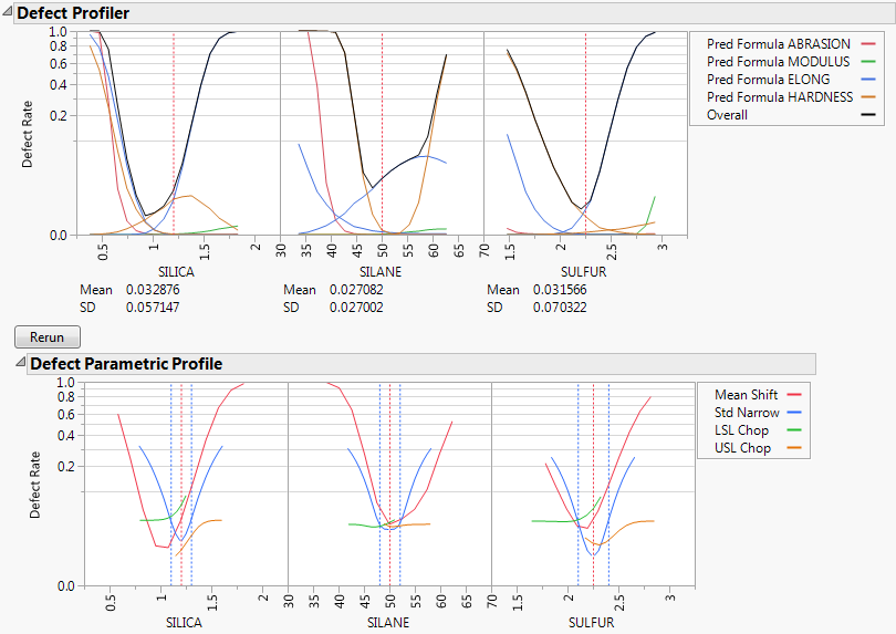
7.	Select Defect Profiler from the Simulator red triangle menu to see the defect profiles. The curves, Means, and SDs will change from simulation to simulation, but will be relatively consistent.

Defect Profiler

Note: Your numbers might differ from those shown in Defect Profiler.

The black curve on each factor shows the defect rate if you could fix that factor at the x-axis value, but leave the other features random.

Look at the curve for SILICA. As its values vary, its defect rate goes from the lowest 0.001 at SILICA=0.95, quickly up to a defect rate of 1 at SILICA=0.4 or 1.8. However, SILICA is itself random. If you imagine integrating the density curve of SILICA with its defect profile curve, you could estimate the average defect rate 0.033, also shown as the Mean for SILICA. This is estimating the overall defect rate shown under the simulation histograms, but by numerically integrating, rather than by the overall simulation. The Means for the other factors are similar. The numbers are not exactly the same. However, we now also get an estimate of the standard deviation of the defect rate with respect to the variation in SILICA. This value (labeled SD) is 0.057. The standard deviation is intimately related to the sensitivity of the defect rate with respect to the distribution of that factor.

Looking at the SDs across the three factors, we see that the SD for SULFUR is higher than the SD for SILICA, which is in turn much higher than the SD for SILANE. This means that to improve the defect rate, improving the distribution in SULFUR should have the greatest effect. A distribution can be improved in three ways: changing its mean, changing its standard deviation, or by chopping off the distribution by rejecting parts that do not meet certain specification limits.

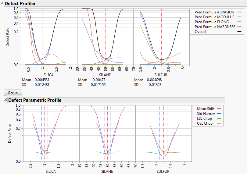
8.	Select Defect Parametric Profile from the Simulator red triangle menu. This command shows how single changes in the factor distribution parameters affect the defect rate.

Defect Parametric Profile

Let’s look closely at the SULFUR situation. You might need to enlarge the graph to see more detail.

First, note that the current defect rate (0.03) is represented in four ways corresponding to each of the four curves.

For the red curve, Mean Shift, the current rate is where the red solid line intersects the vertical red dotted line. The Mean Shift curve represents the change in overall defect rate by changing the mean of SULFUR. One opportunity to reduce the defect rate is to shift the mean slightly to the left. If you use the crosshair tool on this plot, you see that a mean shift reduces the defect rate to about 0.02.

For the blue curve, Std Narrow, the current rate represents where the solid blue line intersects the two dotted blue lines. The Std Narrow curves represent the change in defect rate by changing the standard deviation of the factor. The dotted blue lines represent one standard deviation below and above the current mean. The solid blue lines are drawn symmetrically around the center. At the center, the blue line typically reaches a minimum, representing the defect rate for a standard deviation of zero. That is, if we totally eliminate variation in SULFUR, the defect rate is still around 0.003. This is much better than 0.03. If you look at the other Defect parametric profile curves, you can see that this is better than reducing variation in the other factors, something that we suspected by the SD value for SULFUR.

For the green curve, LSL Chop, there are no interesting opportunities in this example, because the green curve is above current defect rates for the whole curve. This means that reducing the variation by rejecting parts with too-small values for SULFUR will not help.

For the orange curve, USL Chop, there are good opportunities. Reading the curve from the right, the curve starts out at the current defect rate (0.03), then as you start rejecting more parts by decreasing the USL for SULFUR, the defect rate improves. However, moving a spec limit to the center is equivalent to throwing away half the parts, which might not be a practical solution.

Looking at all the opportunities over all the factors, it now looks like there are two good options for a first move: change the mean of SILICA to about 1, or reduce the variation in SULFUR. Because it is generally easier in practice to change a process mean than process variation, the best first move is to change the mean of SILICA to 1.

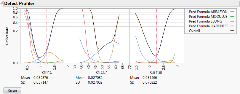
9.	Adjust the Mean of SILICA from 1.2 to 1.0. Click Rerun.

Adjusting the Mean of SILICA

After clicking Rerun, we get a new perspective on defect rates.

Adjusted Defect Rates

Now, the defect rate is down to about 0.004, much improved. Further reduction in the defect rate can occur by continued investigation of the parametric profiles, making changes to the distributions, and rerunning the simulations.

As the defect rate is decreased further, the mean defect rates across the factors become relatively less reliable. The accuracy could be improved by reducing the ranges of the factors in the Profiler a little so that it integrates the distributions better.

This level of fine-tuning is probably not practical, because the experiment that estimated the response surface is probably not at this high level of accuracy. Once the ranges have been refined, you might need to conduct another experiment focusing on the area that you know is closer to the optimum.